回到特征:构建论文推荐器
在数学中,你并不是理解事物,你只是习惯了它们。
—— 约翰·冯·诺依曼(John von Neumann)
当我们最初在图 1-1中引入从数据到结果的路径时,可能还不清楚怎样才能有前进的道路。贯穿全书,我们一直专注于用玩具模型和干净、简单的数据集介绍特征工程的基本原理。这些例子的目的是说明问题和启发思考。
机器学习示例通常展示的是最佳情况和结果。这掩盖了我们迄今在书中描述的路径。既然基础已经打好,我们要离开简单玩具数据的世界,用真实世界的结构化数据集一头扎进特征工程的实践。在逐步推进的每一步中,我们都会考察构成每个特征的原始数据、变换后的特征变成了什么样子,以及我们一路走来做出的权衡。
需要说明的是,我们这个例子的目标并不是为这个数据集构建最好的模型。相反,它旨在演示我们若干技术的实际应用,以及如何更深入地检验和理解每种技术是否正在为人们正在构建的模型提供价值。
基于物品的协同过滤(Item-Based Collaborative Filtering)
我们的任务是用微软学术图谱(Microsoft Academic Graph)数据集的一个子样本构建一个学术论文推荐器。这对于所有正在搜索引文、但尚未发现 Google Scholar 的人来说应该非常有用。以下是关于该数据集的一些相关统计信息:
微软学术图谱数据集
- 它包含 166,192,182 篇唯一论文,可通过 Open Academic Graph 获取。该数据集仅供研究用途。
- 数据集总大小为 104 GB。
- 每条观测有 18 个变量来标识每篇论文,包括论文的标题、摘要、作者、关键词和研究领域。
这个数据集被设计为易于在数据库中存储和访问。它开箱即用并不适合机器学习模型,需要一些初始的数据整理(wrangling)。有些老师喜欢替你省去这一步,直接进入模型和结果来增强你的信心。我们这里没有这种套路。我们从最开始一起出发。
我们最初的方案是把几个变量整理成合适的形状,喂给基于物品的协同过滤(item-based collaborative filtering)。我们将看看能否及时、高效地找到足够相似的论文。
基于物品的协同过滤的起源(The Origins of Item-Based Collaborative Filtering)
这种方法最初由亚马逊开发,作为基于用户的(user-based)产品推荐算法的改进。Sarawar 等人(2001)详细介绍了把推荐器的视角从用户切换到物品所带来的挑战和好处。
基于物品的协同过滤根据物品之间的相似度提供推荐。它分两个阶段工作:首先计算物品之间的相似度分数,然后对所有分数排序,找出相似度最高的前 N 个物品推荐。
构建基于物品的推荐器
基于物品的推荐器执行三项任务:
- 概括关于某个"东西"或物品的信息。
- 对所有其他物品打分,找出"像"这个物品的那些。
- 返回排序后的分数 + 物品。
第一轮:数据导入、清洗与特征解析(First Pass: Data Import, Cleaning, and Feature Parsing)
像所有好的科学实验一样,我们从假设开始。在这种情况下,我们假设大约在同一时间发表、研究领域相似的论文对用户最有用。我们将采用一种朴素的方法,从整个数据集的子样本中解析出这些领域。在生成简单的稀疏数组之后,我们让整个物品数组通过一个基于物品的协同过滤器,看看是否得到好结果。
基于物品的协同过滤器依赖相似度分数来比较物品。在这种情况下,余弦相似度(cosine similarity)为两个非零向量提供了合理的比较。下面的例子实际使用的是余弦距离(cosine distance),它是正空间中余弦相似度的补,即:
\[ D_C(A, B) = 1 - S_C(A, B) \]其中 \(D_C\) 是余弦距离,\(S_C\) 是余弦相似度。
学术论文推荐器:朴素方法(Naive Approach)
我们旅程的第一步是导入并检查数据集。在示例 9-1中,我们通过限制初始导入后可用的字段来限定实验范围。如图 图 9-1 所示,这些字段仍然蕴含丰富的可能性。
示例 9-1:导入并过滤数据
>>> import pandas as pd
>>> model_df = pd.read_json('data/mag_papers_0/mag_subset20K.txt', lines=True)
>>> model_df.shape
(20000, 19)
>>> model_df.columns
Index(['abstract', 'authors', 'doc_type', 'doi', 'fos', 'id', 'issue',
'keywords', 'lang', 'n_citation', 'page_end', 'page_start', 'publisher',
'references', 'title', 'url', 'venue', 'volume', 'year'],
dtype='object')
# filter out non-English articles and focus on a few variables
>>> model_df = model_df[model_df.lang == 'en']
... .drop_duplicates(subset='title', keep='first')
... .drop(['doc_type', 'doi', 'id', 'issue', 'lang', 'n_citation',
... 'page_end', 'page_start', 'publisher', 'references',
... 'url', 'venue', 'volume'], axis=1)
>>> model_df.shape
(10399, 6)
表 9-1 最好地总结了还需要怎样的进一步整理,才能把原始数据处理成更适合模型的形状。列表和字典适合存储数据,但不经过一些拆解就不整洁,也不适合机器学习(Wickham,2014)。
| 字段名 | 描述 | 字段类型 | NaN 数量 |
|---|---|---|---|
| abstract | 论文摘要 | 字符串(string) | 4393 |
| authors | 作者姓名和单位 | 字典列表,键 = name、org | 1 |
| fos | 研究领域 | 字符串列表 | 1733 |
| keywords | 关键词 | 字符串列表 | 4294 |
| title | 论文标题 | 字符串 | 0 |
| year | 发表年份 | 整数(int) | 0 |
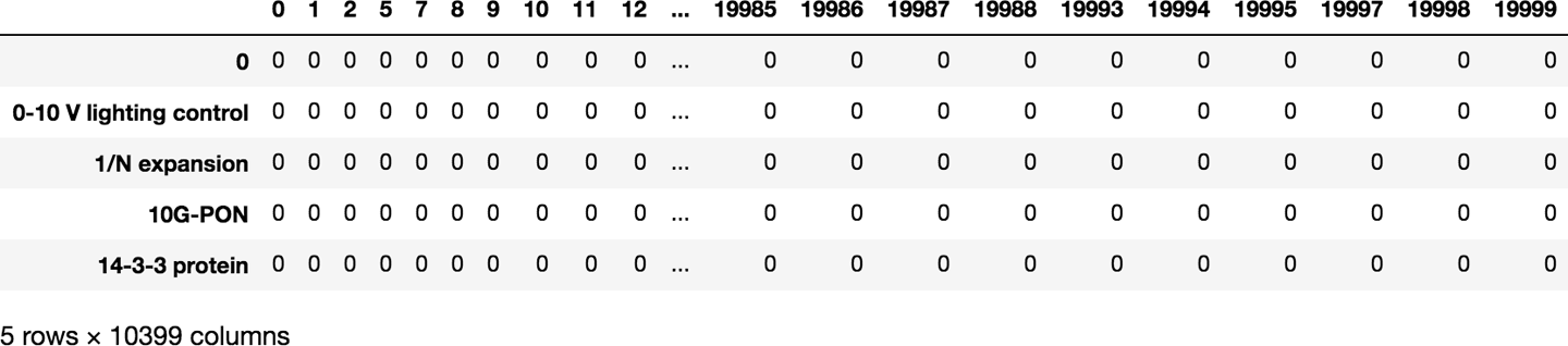
在示例 9-2中,我们首先关注两个字段,把它们从列表和整数变换成一个特征数组,如图 图 9-2 所示。
示例 9-2:协同过滤第 1 阶段:构建物品特征矩阵
>>> unique_fos = sorted(list({feature
... for paper_row in model_df.fos.fillna('0')
... for feature in paper_row}))
>>> unique_year = sorted(model_df['year'].astype('str').unique())
>>> def feature_array(x, var, unique_array):
...     row_dict = {}
...     for i in x.index:
...         var_dict = {}
...         for j in range(len(unique_array)):
...             if type(x[i]) is list:
...                 if unique_array[j] in x[i]:
...                     var_dict.update({var + '_' + unique_array[j]: 1})
...                 else:
...                     var_dict.update({var + '_' + unique_array[j]: 0})
...             else:
...                 if unique_array[j] == str(x[i]):
...                     var_dict.update({var + '_' + unique_array[j]: 1})
...                 else:
...                     var_dict.update({var + '_' + unique_array[j]: 0})
...         row_dict.update({i: var_dict})
...     feature_df = pd.DataFrame.from_dict(row_dict, dtype='str').T
...     return feature_df
>>> year_features = feature_array(model_df['year'], unique_year)
>>> fos_features = feature_array(model_df['fos'], unique_fos)
>>> first_features = fos_features.join(year_features).T
>>> from sys import getsizeof
>>> print('Size of first feature array: ', getsizeof(first_features))
Size of first feature array: 2583077234

我们现在成功地把一个相对较小的数据集——大约 1 万行原始数据——变成了 2.5 GB 的特征。但这条路对于快速、迭代式的探索来说太笨重了。我们需要更快的方法,产生消耗更少计算资源和实验时间的特征。
不过,目前让我们先看看当前特征在下一阶段(示例 9-3)能否给出好的推荐。我们把"好"的推荐定义为看起来与输入相似的论文。
示例 9-3:协同过滤第 2 阶段:搜索相似物品
>>> from scipy.spatial.distance import cosine
>>> def item_collab_filter(features_df):
...     item_similarities = pd.DataFrame(index=features_df.columns,
...                                      columns=features_df.columns)
...     for i in features_df.columns:
...         for j in features_df.columns:
...             item_similarities.loc[i][j] = 1 - cosine(features_df[i],
...                                                      features_df[j])
...     return item_similarities
>>> first_items = item_collab_filter(first_features.loc[:, 0:1000])
为什么只用两个特征计算物品相似度要花这么长时间?因为我们使用嵌套 for 循环对 10,399 × 1,000 矩阵做点积。随着我们向模型添加更多的观测,每次循环的时间也会增加。请记住,这只是可用数据集的一个子集,而且只过滤出英文论文。当我们越来越接近"好"的结果时,我们需要回到更大的集合上测试我们最好的结果。
怎样才能更快?既然我们一次只需要一个结果,我们可以修改函数,一次只计算一个物品,并指定想要的前 N 个结果。随着实验的继续,我们稍后会这样做。现在,看看完整的特征空间是有用的,可以理解在真实世界数据集上进行暴力破解(brute-force)时迭代工作带来的影响。
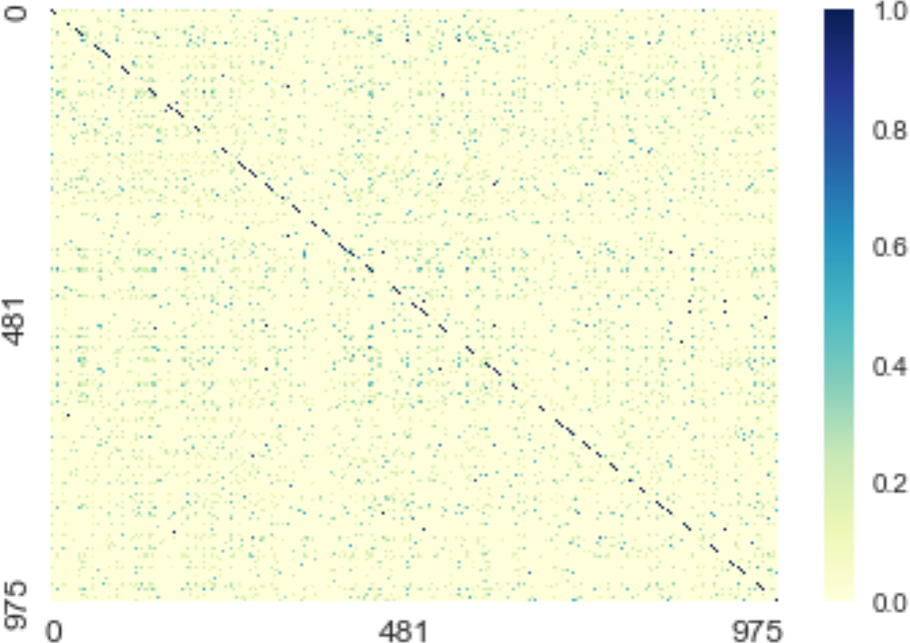
我们需要更好地了解这些特征将如何帮助我们获得好的推荐。我们有足够的观测继续前进吗?让我们绘制一个热力图(示例 9-4),看看是否有彼此相似的论文。图 9-3 显示了结果。
示例 9-4:论文推荐热力图
>>> import matplotlib.pyplot as plt
>>> import seaborn as sns
>>> import numpy as np
>>> %matplotlib inline
>>> sns.set()
>>> ax = sns.heatmap(first_items.fillna(0),
...                 vmin=0, vmax=1,
...                 cmap="YlGnBu",
...                 xticklabels=250, yticklabels=250)
>>> ax.tick_params(labelsize=12)
较暗的像素表示彼此相似的物品。暗色对角线表明余弦相似度正确地指出了每篇论文与自身最相似。然而,由于我们某个特征存在大量 NaN,这条线沿对角线是断开的。我们可以看到,虽然大多数物品彼此不相似——也就是说,我们的数据集相当多样——但仍有一些得分较高的候选者。从定性角度看,它们可能是也可能不是好的推荐,但至少我们可以看到我们的方法并非完全离谱。

示例 9-5 展示了如何把这些物品相似度转化为推荐。好消息是,我们仍然有各种各样的特征可用,改进空间很大。
示例 9-5:基于物品的协同过滤推荐
>>> def paper_recommender(paper_ix, items_df):
...     print('Based on the paper: \n index = ', paper_ix)
...     print(model_df.iloc[paper_ix])
...     top_results = items_df.loc[paper_ix].sort_values(ascending=False).head(4)
...     print(' \n Top three results: ')
...     order = 1
...     for i in top_results.index.tolist()[-3:]:
...         print(order, '. Paper index = ', i)
...         print('Similarity score: ', top_results[i])
...         print(model_df.iloc[i], ' \n ')
...         if order < 5: order += 1
>>> paper_recommender(2, first_items)
Based on the paper:
index =  2
abstract                                                  NaN
authors     [{'name': 'Jovana P. Lekovich', 'org': 'Weill ...
fos                                                       NaN
keywords                                                  NaN
title       Should endometriosis be an indication for intr...
year                                                     2015
Name: 2, dtype: object
Top three results:
1 . Paper index =  2
Similarity score:  1.0
abstract                                                  NaN
authors     [{'name': 'Jovana P. Lekovich', 'org': 'Weill ...
fos                                                       NaN
keywords                                                  NaN
title       Should endometriosis be an indication for intr...
year                                                     2015
Name: 2, dtype: object
2 . Paper index =  292
Similarity score:  1.0
abstract                                                  NaN
authors     [{'name': 'John C. Newton'}, {'name': 'Beers M...
fos         [Wide area multilateration, Maneuvering speed,...
keywords                                                  NaN
title                    Automatic speed control for aircraft
year                                                     1955
Name: 561, dtype: object
3 . Paper index =  593
Similarity score:  1.0
abstract    This paper demonstrates that on-site greywater...
authors     [{'name': 'Eran Friedler', 'org': 'Division of...
fos         [Public opinion, Environmental Engineering, Wa...
keywords    [economic analysis, tratamiento desperdicios, ...
title       The water saving potential and the socio-econo...
year                                                     2008
Name: 1152, dtype: object
哎呀。好消息是,返回的最相似论文正是我们正在寻找的那篇。坏消息是,接下来两篇论文似乎与我们最初的搜索不太接近,即使对我们选择的特征来说也是如此。
“是的,是的,“你可能会说,“但这是大数据时代!这会解决我们的问题!我们能不能干脆喂入更多数据以获得更好的结果?“也许吧。但即使是大数据也无法弥补糟糕的数据和工程选择。
我们目前的暴力破解方法对于聪明、迭代式的工程来说太慢了。让我们尝试一些新的特征工程技巧,看看能否加快计算时间,找到更好的特征和更好的结果搜索方式。
第二轮:更多工程与更智能的模型(Second Pass: More Engineering and a Smarter Model)
最初的方法——创建一个大而稀疏的数组,然后把它塞进过滤器——可以在很多方面加以改进。接下来的步骤将专门致力于把更好的技术应用于最初的两个特征,并改进基于物品的协同过滤方法,以便更快地迭代。
首先,是时候为假设中的那两个变量尝试一些出色的特征工程技巧了。深入研究已经开发出的特征后,我们可以选择适合每种变量类型的技术,把它转换成推荐系统所需的"更好"特征。
学术论文推荐器:第二轮(Academic Paper Recommender: Take 2)
让我们先关注 year 字段。在“量化或分箱”一节中,我们回顾过:对于使用相似度度量的方法来说,把原始计数直接用作特征可能带来问题。示例 9-6(以及图 9-5)将检验我们如何转换 'year',使其更好地适配已选定的模型。
示例 9-6:定宽分箱 + 哑变量编码(第 1 部分)
>>> print("Year spread: ", model_df['year'].min(), " - ", model_df['year'].max())
>>> print("Quantile spread: \n ", model_df['year'].quantile([0.25, 0.5, 0.75]))
Year spread:  1831  -  2017
Quantile spread:
0.25    1990.0
0.50    2005.0
0.75    2012.0
Name: year, dtype: float64
# plot years to see the distribution
>>> fig, ax = plt.subplots()
>>> model_df['year'].hist(ax=ax,
... bins=model_df['year'].max() - model_df['year'].min())
>>> ax.tick_params(labelsize=12)
>>> ax.set_xlabel('Year Count', fontsize=12)
>>> ax.set_ylabel('Occurrence', fontsize=12)
从偏态分布(图 9-5)可以看出,这是分箱的绝佳候选。
分箱将基于变量内部的取值范围,而不是特征的唯一数量。为了进一步缩小特征空间,我们将对生成的分箱做哑变量编码(参见示例 9-7)。Pandas 可以用内置函数同时完成这两件事。这些方法会让我们的结果易于解释,因此我们可以在继续之前快速检查转换后的特征(参见图 9-6)。
示例 9-7:定宽分箱 + 哑变量编码(第 2 部分)
# binning here (by 10 years) reduces the year feature space from 156 to 19
>>> bins = int(round((model_df['year'].max() - model_df['year'].min()) / 10))
>>> temp_df = pd.DataFrame(index=model_df.index)
>>> temp_df['yearBinned'] = pd.cut(model_df['year'].tolist(), bins, precision=0)
>>> X_yrs = pd.get_dummies(temp_df['yearBinned'])
>>> X_yrs.columns.categories
IntervalIndex([(1831.0, 1841.0], (1841.0, 1851.0], (1851.0, 1860.0],
(1860.0, 1870.0], (1870.0, 1880.0] ... (1968.0, 1978.0],
(1978.0, 1988.0], (1988.0, 1997.0], (1997.0, 2007.0],
(2007.0, 2017.0]]
closed='right',
dtype='interval[float64]')
# plot the new distribution
>>> fig, ax = plt.subplots()
>>> X_yrs.sum().plot.bar(ax=ax)
>>> ax.tick_params(labelsize=8)
>>> ax.set_xlabel('Binned Years', fontsize=12)
>>> ax.set_ylabel('Counts', fontsize=12)
我们通过按十年分箱,保留了原始变量的潜在分布。如果我们希望使用某种能从不同分布中受益的方法,就可以调整分箱的选择,改变这个变量呈现在模型面前的方式。由于我们用的是余弦相似度,这样处理没有问题。让我们继续处理最初纳入模型的另一个特征。
fields-of-study 特征空间对原始模型的大小和处理时间贡献巨大。
让我们看看已经完成的工作。在第一轮中,我们通过解析字符串列表,创建了一个"短语袋”(bag-of-phrases)。既然我们已经有了一个有用的稀疏数组,就可以专注于使用更高效的数据类型。示例 9-8演示了把 Pandas DataFrame 转换为 NumPy 稀疏数组如何影响计算时间。
示例 9-8:将 bag-of-phrases 的 pd.Series 转换为 NumPy 稀疏数组
>>> X_fos = fos_features.values
# We can see how this will make a difference in the future by looking
# at the size of each
>>> print('Our pandas Series, in bytes: ', getsizeof(fos_features))
>>> print('Our hashed numpy array, in bytes: ', getsizeof(X_fos))
Our pandas Series, in bytes:  2530632380
Our hashed numpy array, in bytes:  112
好多了!把它们重新组合起来:我们将特征拼接在一起(示例 9-9),并利用 scikit-learn 的余弦相似度函数重新运行推荐器(示例 9-10),看看结果是否有所改善。我们还会一次只关注一个物品,以缩短计算时间。
示例 9-9:协同过滤第 1 + 2 阶段:构建物品特征矩阵,搜索相似物品
>>> second_features = np.append(X_fos, X_yrs, axis=1)
>>> print("The power of feature engineering saves us, in bytes: ",
... getsizeof(first_features) - getsizeof(second_features))
The power of feature engineering saves us, in bytes:  168066769
>>> from sklearn.metrics.pairwise import cosine_similarity
>>> def piped_collab_filter(features_matrix, index, top_n):
... item_similarities =
\
... 1 - cosine_similarity(features_matrix[index:index + 1],
... features_matrix).flatten()
... related_indices =
\
... [i for i in item_similarities.argsort()[::-1] if i != index]
... return [(index, item_similarities[index])
... for index in related_indices
... ][0:top_n]
示例 9-10:基于物品的协同过滤推荐:第二轮
>>> def paper_recommender(items_df, paper_ix, top_n):
... if paper_ix in model_df.index:
... print('Based on the paper:')
... print('Paper index = ', model_df.loc[paper_ix].name)
... print('Title :', model_df.loc[paper_ix]['title'])
... print('FOS :', model_df.loc[paper_ix]['fos'])
... print('Year :', model_df.loc[paper_ix]['year'])
... print('Abstract :', model_df.loc[paper_ix]['abstract'])
... print('Authors :', model_df.loc[paper_ix]['authors'], ' \n ')
... # define the location index for the DataFrame index requested
... array_ix = model_df.index.get_loc(paper_ix)
... top_results = piped_collab_filter(items_df, array_ix, top_n)
... print(' \n Top', top_n, 'results: ')
... order = 1
... for i in range(len(top_results)):
... print(order, '. Paper index = ',
... model_df.iloc[top_results[i][0]].name)
... print('Similarity score: ', top_results[i][1])
... print('Title :', model_df.iloc[top_results[i][0]]['title'])
... print('FOS :', model_df.iloc[top_results[i][0]]['fos'])
... print('Year :', model_df.iloc[top_results[i][0]]['year'])
... print('Abstract :', model_df.iloc[top_results[i][0]]['abstract'])
... print('Authors :', model_df.iloc[top_results[i][0]]['authors'],
... ' \n ')
... if order < top_n: order += 1
... else:
... print('Whoops! Choose another paper. Try something from here: \n ',
... model_df.index[100:200])
>>> paper_recommender(second_features, 2, 3)
Based on the paper:
Paper index =  2
Title : Should endometriosis be an indication for intracytoplasmic sperm inject ...
FOS : nan
Year : 2015
Abstract : nan
Authors : [{'name': 'Jovana P. Lekovich', 'org': 'Weill Cornell Medical College, ...
Top 3 results:
1 . Paper index =  10055
Similarity score:  1.0
Title : [Diagnosis of cerebral tumors; comparative studies on arteriography, ...
FOS : ['Radiology', 'Pathology', 'Surgery']
Year : 1953
Abstract : nan
Authors : [{'name': 'Antoine'}, {'name': 'Lepoire'}, {'name': 'Schoumacker'}]
2 . Paper index =  11771
Similarity score:  1.0
Title : A Study of Special Functions in the Theory of Eclipsing Binary Systems
FOS : ['Contact binary']
Year : 1981
Abstract : nan
Authors : [{'name': 'Filaretti Zafiropoulos', 'org': 'University of Manchester'}]
3 . Paper index =  11773
Similarity score:  1.0
Title : Studies of powder flow using a recording powder flowmeter and measure ...
FOS : nan
Year : 1985
Abstract : This paper describes the utility of the dynamic measurement of the ...
Authors : [{'name': 'Ramachandra P. Hegde', 'org': 'Department of Pharmacy, ...
说实话,我不认为我们的特征选择效果很好。这些字段里有大量缺失数据。让我们继续走下去,看看能否选择信息更丰富的特征。
找准位置(Finding Your Place)
在 Pandas DataFrame 与 NumPy 矩阵之间转换会让索引变得棘手——索引的大小相同,但索引的分配并不一致。Pandas 借助 .iloc、.loc 和 .get_loc 来协助处理,正如我们在示例 9-11中展示的:
.loc基于原始 Pandas DataFrame 返回索引,让我们能够引用特定的论文。.iloc使用整数位置,与 NumPy 数组的索引一致。.get_loc帮助我们在已知 DataFrame 索引的情况下找到整数位置。
示例 9-11:转换过程中保持索引分配
>>> model_df.loc[21]
abstract    A microprocessor includes hardware registers t...
authors                      [{'name': 'Mark John Ebersole'}]
fos         [Embedded system, Parallel computing, Computer...
keywords                                                  NaN
title       Microprocessor that enables ARM ISA program to...
year                                                     2013
Name: 21, dtype: object
>>> model_df.iloc[21]
abstract                                                  NaN
authors     [{'name': 'Nicola M. Heller'}, {'name': 'Steph...
fos         [Biology, Medicine, Post-transcriptional regul...
keywords    [glucocorticoids, post transcriptional regulat...
title       Post-transcriptional regulation of eotaxin by ...
year                                                     2002
Name: 30, dtype: object
>>> model_df.index.get_loc(30)
21
第三轮:更多特征 = 更多信息(Third Pass: More Features = More Information)
到目前为止,我们的实验并不支持最初的假设,即 year 和 fields-of-study 足以推荐出相似的论文。此时,我们有几个选择:
- 上传更多原始数据集,看看能否得到更好的结果。
- 花更多时间探索数据,检查我们是否拥有足够密集的集合来提供好的推荐。
- 在当前模型上继续迭代,添加更多特征。
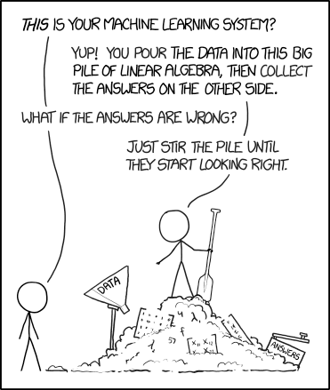
第一个选择假设问题出在我们对数据的抽样上。情况或许如此,但这就像图 9-4 的类比——搅动数据堆以期获得更好的结果。
第二个选择能让我们更好地了解底层的原始数据。随着探索过程中特征与模型选择的决策不断变化,这一步应该被持续重新审视。这里选取的初始子样本正是这一步的体现。由于数据集中还有更多可用变量,我们暂时还不会回到这一步。
这就剩下了第三个选择:在当前模型上继续前进,添加更多特征。为每个物品提供更多信息可以提高相似度得分,带来更好的推荐。
基于最初的探索,接下来的步骤将聚焦于信息量最大的字段:abstract 和 authors。
学术论文推荐器:第三轮(Academic Paper Recommender: Take 3)
回顾第 4 章,我们可以看到 abstract 是 tf-idf 的绝佳候选,它能过滤掉噪声,找出突出的关联词。我们在示例 9-12中这样做。
示例 9-12:停用词 + tf-idf
# need to fill in NaN for sklearn use in future
>>> filled_df = model_df.fillna('None')
>>> from sklearn.feature_extraction.text import TfidfVectorizer
>>> vectorizer = TfidfVectorizer(sublinear_tf=True, max_df=0.5,
... stop_words='english')
>>> X_abstract = vectorizer.fit_transform(filled_df['abstract'])
>>> third_features = np.append(second_features, X_abstract.toarray(), axis=1)
authors 字段杂乱且不均匀,我们可以把它整理成字典,再送入 one-hot 编码器处理,从而降低计算负荷,如示例 9-13所示。
示例 9-13:使用 scikit-learn 的 DictVectorizer 进行 one-hot 编码
>>> authors_list = []
>>> for row in filled_df.authors.itertuples():
... # create a dictionary from each Series index
... if type(row.authors) is str:
... y = {'None': row.Index}
... if type(row.authors) is list:
... # add these keys + values to our running dictionary
... y = dict.fromkeys(row.authors[0].values(), row.Index)
... authors_list.append(y)
>>> authors_list[0:5]
[{'None': 0},
{'Ahmed M. Alluwaimi': 1},
{'Jovana P. Lekovich': 2, 'Weill Cornell Medical College, New York, NY': 2},
{'George C. Sponsler': 5},
{'M. T. Richards': 7}]
>>> from sklearn.feature_extraction import DictVectorizer
>>> v = DictVectorizer(sparse=False)
>>> D = authors_list
>>> X_authors = v.fit_transform(D)
>>> fourth_features = np.append(third_features, X_authors, axis=1)
是时候与推荐器核对一下,看看这些新特征效果如何了。示例 9-14 显示了结果。
示例 9-14:基于物品的协同过滤推荐:第三轮
>>> paper_recommender(fourth_features, 2, 3)
Based on the paper:
Paper index =  2
Title : Should endometriosis be an indication for intracytoplasmic sperm inject ...
FOS : nan
Year : 2015
Abstract : nan
Authors : [{'name': 'Jovana P. Lekovich', 'org': 'Weill Cornell Medical College, ...
Top 3 results:
1 . Paper index =  10055
Similarity score:  1.0
Title : [Diagnosis of cerebral tumors; comparative studies on arteriography, ...
FOS : ['Radiology', 'Pathology', 'Surgery']
Year : 1953
Abstract : nan
Authors : [{'name': 'Antoine'}, {'name': 'Lepoire'}, {'name': 'Schoumacker'}]
2 . Paper index =  5601
Similarity score:  1.0
Title : 633 Survival after coronary revascularization, with and without mitral ...
FOS : ['Cardiology']
Year : 2005
Abstract : nan
Authors : [{'name': 'J.B. Le Polain De Waroux'}, {'name': 'Anne-Catherine ...
3 . Paper index =  12256
Similarity score:  1.0
Title : Nucleotide Sequence and Analysis of an Insertion Sequence from Bacillus ...
FOS : ['Biology', 'Molecular biology', 'Insertion sequence', 'Nucleic acid ...
Year : 1994
Abstract : A 5.8-kb DNA fragment encoding the  cryIC  gene from  Bacillus thur...
Authors : [{'name': 'Geoffrey P. Smith'}, {'name': 'David J. Ellar'}, {'name': ...
即使考虑到某些字段中的缺失数据,上一轮特征工程给出的前三名结果也在把我们引向医学领域的其他论文。
这个数据集所覆盖的论文范围很广;例如,随机抽样的一些论文暴露出诸如"耦合常数”(Coupling constant)、“蒸散发”(Evapotranspiration)、“哈希函数”(Hash function)、“IVMS”、“冥想”(Meditation)、“帕累托分析”(Pareto analysis)、“第二代小波变换”(Second-generation wavelet transform)、“滑动”(Slip)和"旋涡星系”(Spiral galaxy)等研究领域。考虑到 1 万+ 篇论文列出了 7,604 个独特的研究领域,这些最终结果似乎在朝着正确的方向前进。我们可以确信,我们的工作正一步步走向一个有用的模型。
继续在更多文本变量上迭代——比如找出论文标题中的名词短语,或对关键词做词干提取——可以让我们更接近"最佳"推荐。
需要指出的是,这里对"最佳"的定义是所有推荐器和搜索引擎共同追求的圣杯。我们在寻找用户觉得最有帮助的东西,而它未必直接由数据呈现。特征工程让我们能够把显著特征抽象成某种表示,使算法既能揭示其中显式的信息,也能揭示隐式的信息。
小结(Summary)
如你所见,为机器学习构建模型很容易。但构建好用的模型、产出有用的结果,需要时间和投入。我们在这里走过了杂乱无章的全程:审视一组可能的变量,试验不同的特征工程方法,以获得更好的结果。我们在此定义的"更好”,不仅指训练和测试的良好表现,还包括缩小模型的规模、缩短我们在不同实验间迭代所需的时间。
我们在本书开头谈到:精通一门学科,来自于深入学习其中起作用的原理,从而获得直觉,以便有效地把知识付诸实践。我们希望我们的工作为你提供了必要的工具,让你变得更高效、更有效;同时,也加深了你在数学与计算层面上的理解——特征工程是开发有用的机器学习模型所必备的技能。
参考文献(Bibliography)
Sarwar, Badrul, George Karypis, Joseph Konstan, and John Riedl. “Item-Based Collaborative Filtering Recommendation Algorithms.” Proceedings of the 10th International Conference on the World Wide Web (2001) 285-295.
Sinha, Arnab, Zhihong Shen, Yang Song, Hao Ma, Darrin Eide, Bo-June (Paul) Hsu, and Kuansan Wang. “An Overview of Microsoft Academic Service (MAS) and Applications.” Proceedings of the 24th International Conference on the World Wide Web (2015): 243-246.
Tang, Jie, Jing Zhang, Limin Yao, Juanzi Li, Li Zhang, and Zhong Su. “ArnetMiner: Extraction and Mining of Academic Social Networks.” Proceedings of the 14th ACM SIGKDD International Conference on Knowledge Discovery and Data Mining (2008): 990-998.
Wickham, Hadley. “Tidy Data.” The Journal of Statistical Software 59 (2014).