集成与堆叠
当我们听到这两个词时,脑海中浮现的第一件事就是它们与线上/线下机器学习竞赛(machine learning competitions)有关。这在几年前确实如此,但随着计算能力的进步和更便宜的虚拟实例(virtual instances)的出现,人们现在甚至开始在工业界使用集成模型(ensemble models)。例如,部署多个神经网络(neural network)并在 500ms 以内的响应时间内实时提供服务是很容易的。有时候,一个巨大的神经网络或大型模型也可以被几个体积小、性能与大型模型相当且速度快一倍的小模型所取代。如果是这种情况,你会选择哪个(些)模型?就我个人而言,我会更喜欢多个小模型,它们更快,并且能给出与更大更慢的模型相同的性能。请记住,小模型也更容易、更快地调优。
集成(ensembling)无非就是不同模型的组合。模型可以通过它们的预测/概率(predictions/probabilities)来组合。组合模型最简单的方法就是做平均(average)。
\[ \text{Ensemble Probabilities} = \frac{M1_{\text{proba}} + M2_{\text{proba}} + \ldots + Mn_{\text{Proba}}}{n} \]这很简单,却是组合模型最有效的方法。在简单平均(simple averaging)中,所有模型的权重相等。对于任何组合方法,你都需要记住一件事:你应该总是组合彼此不同的模型的预测/概率。简单地说,组合相关性不高的模型,效果要好于组合彼此高度相关的模型。
如果你没有概率,你也可以组合预测。最简单的做法是投票(vote)。假设我们正在做一个三类的多分类(multi-class classification)问题:类别 0、1 和 2。
- [0, 0, 1]:得票最高的类别:0
- [0, 1, 2]:得票最高的类别:无(随机选一个)
- [2, 2, 2]:得票最高的类别:2
下面这些简单的函数可以完成这些简单操作。
import numpy as np


def mean_predictions(probas):
    """
    Create mean predictions

    :param probas: 2-d array of probability values
    :return: mean probability
    """
    return np.mean(probas, axis=1)


def max_voting(preds):
    """
    Create mean predictions

    :param probas: 2-d array of prediction values
    :return: max voted predictions
    """
    idxs = np.argmax(preds, axis=1)
    return np.take_along_axis(preds, idxs[:, None], axis=1)
请注意,probas 的每一列只有一个概率(即二分类(binary classification),通常指类别 1 的概率)。因此每一列就是一个新模型。类似地,对于 preds,每一列都是来自不同模型的预测。这两个函数都假设输入是一个二维 numpy 数组。你可以根据自己的需求修改它。例如,你可能为每个模型都有一个二维概率数组。在这种情况下,函数会稍有变化。组合多个模型的另一种方法是按其概率的排名(ranks)。当所关注的指标是曲线下面积(AUC, area under curve)时,这种组合方式效果很好,因为 AUC 完全关乎样本的排序。
def rank_mean(probas):
    """
    Create mean predictions using ranks

    :param probas: 2-d array of probability values
    :return: mean ranks
    """
    ranked = []
    for i in range(probas.shape[1]):
        rank_data = stats.rankdata(probas[:, i])
        ranked.append(rank_data)

    ranked = np.column_stack(ranked)
    return np.mean(ranked, axis=1)
请注意,在 scipy 的 rankdata 中,排名从 1 开始。
为什么这类集成会有效?让我们看图 1。
Figure 1: Three people guessing the height of an elephant
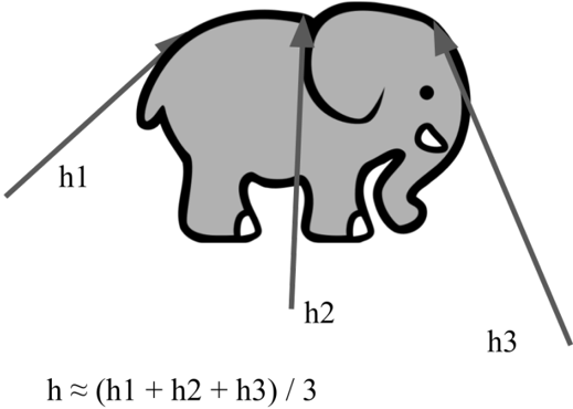
图 1 表明,如果三个人在猜测一头大象的身高,真实身高会非常接近三个人猜测的平均值。假设这些人能够猜得非常接近大象的真实身高。接近的估计意味着存在误差,但当我们对三个预测取平均时,这个误差可以被最小化。这就是对多个模型取平均背后的主要思想。
概率也可以通过权重来组合。
\[ \text{Final Probabilities} = w_1 \times M1_{\text{proba}} + w_2 \times M2_{\text{proba}} + \ldots + w_n \times Mn_{\text{proba}} \]其中 \(w_1 + w_2 + w_3 + \ldots + w_n = 1.0\)
例如,如果你有一个随机森林(random forest)模型,它的 AUC 非常高,还有一个逻辑回归(logistic regression)模型,AUC 略低一些,你可以用 70% 给随机森林、30% 给逻辑回归的方式来组合它们。那么,我是怎么得出这些数字的呢?让我们再加入一个模型,比如说现在我们还有一个 xgboost 模型,它的 AUC 高于随机森林。现在我会按 3:2:1 的比例组合它们,即 xgboost : random forest : logistic regression。很简单,对吧?得出这些数字是轻而易举的事。让我们看看怎么做。
假设我们有三个猴子和三个旋钮,旋钮的值在 0 到 1 之间。这些猴子转动旋钮,我们在它们每次转到的值处计算 AUC 分数。最终,猴子们会找到一个能给出最佳 AUC 的组合。是的,这就是随机搜索(random search)!在进行这类搜索之前,你必须记住集成最重要的两条规则。
集成的第一条规则:在开始集成之前,你总是要先创建折(folds)。
集成的第二条规则:在开始集成之前,你总是要先创建折。
是的。这就是最重要的两条规则,而且,我写的内容没有错误。第一步是创建折。为了简单起见,我们假设把数据分成两部分:折 1 和折 2。请注意,这样做只是为了便于解释。在真实场景中,你应该创建更多的折。
现在,我们在折 1 上训练随机森林模型、逻辑回归模型和 xgboost 模型,并在折 2 上做预测。之后,我们在折 2 上从头训练这些模型,并在折 1 上做预测。这样,我们就为所有训练数据创建了预测。现在,为了组合这些模型,我们取出折 1 以及折 1 的所有预测,创建一个优化函数,试图找到最佳的权重,以便相对于折 2 的目标最小化误差或最大化 AUC。所以,我们有点像是在折 1 上训练一个优化模型,以三个模型的预测概率为输入,并在折 2 上评估它。让我们先看一个类,我们可以用它来找到多个模型的最佳权重,以优化 AUC(或一般意义上的任何预测-指标组合)。
import numpy as np
from functools import partial
from scipy.optimize import fmin
from sklearn import metrics


class OptimizeAUC:
    """
    Class for optimizing AUC.

    This class is all you need to find best weights for any model and for any
    metric and for any types of predictions. With very small changes, this class
    can be used for optimization of weights in ensemble models of _any_ type of
    predictions
    """

    def __init__(self):
        self.coef_ = 0

    def _auc(self, coef, X, y):
        """
        This functions calulates and returns AUC.

        :param coef: coef list, of the same length as number of models
        :param X: predictions, in this case a 2d array
        :param y: targets, in our case binary 1d array
        """
        # multiply coefficients with every column of the array
        # with predictions.
        # this means: element 1 of coef is multiplied by column 1
        # of the prediction array, element 2 of coef is multiplied
        # by column 2 of the prediction array and so on!
        x_coef = X * coef

        # create predictions by taking row wise sum
        predictions = np.sum(x_coef, axis=1)

        # calculate auc score
        auc_score = metrics.roc_auc_score(y, predictions)

        # return negative auc
        return -1.0 * auc_score

    def fit(self, X, y):
        # remember partial from hyperparameter optimization chapter?
        loss_partial = partial(self._auc, X=X, y=y)

        # dirichlet distribution. you can use any distribution you want
        # to initialize the coefficients
        # we want the coefficients to sum to 1
        initial_coef = np.random.dirichlet(np.ones(X.shape[1]), size=1)

        # use scipy fmin to minimize the loss function, in our case auc
        self.coef_ = fmin(loss_partial, initial_coef, disp=True)

    def predict(self, X):
        # this is similar to _auc function
        x_coef = X * self.coef_
        predictions = np.sum(x_coef, axis=1)
        return predictions
让我们看看如何使用它,并与简单平均进行比较。
import xgboost as xgb
from sklearn.datasets import make_classification
from sklearn import ensemble
from sklearn import linear_model
from sklearn import metrics
from sklearn import model_selection

# make a binary classification dataset with 10k samples
# and 25 features
X, y = make_classification(n_samples=10000, n_features=25)

# split into two folds (for this example)
xfold1, xfold2, yfold1, yfold2 = model_selection.train_test_split(
    X, y, test_size=0.5, stratify=y
)

# fit models on fold 1 and make predictions on fold 2
# we have 3 models:
# logistic regression, random forest and xgboost
logreg = linear_model.LogisticRegression()
rf = ensemble.RandomForestClassifier()
xgbc = xgb.XGBClassifier()

# fit all models on fold 1 data
logreg.fit(xfold1, yfold1)
rf.fit(xfold1, yfold1)
xgbc.fit(xfold1, yfold1)

# predict all models on fold 2
# take probability for class 1
pred_logreg = logreg.predict_proba(xfold2)[:, 1]
pred_rf = rf.predict_proba(xfold2)[:, 1]
pred_xgbc = xgbc.predict_proba(xfold2)[:, 1]

# create an average of all predictions
# that is the simplest ensemble
avg_pred = (pred_logreg + pred_rf + pred_xgbc) / 3

# a 2d array of all predictions
fold2_preds = np.column_stack(
    (pred_logreg, pred_rf, pred_xgbc, avg_pred)
)

# calculate and store individual AUC values
aucs_fold2 = []
for i in range(fold2_preds.shape[1]):
    auc = metrics.roc_auc_score(yfold2, fold2_preds[:, i])
    aucs_fold2.append(auc)

print(f"Fold-2: LR AUC = {aucs_fold2[0]}")
print(f"Fold-2: RF AUC = {aucs_fold2[1]}")
print(f"Fold-2: XGB AUC = {aucs_fold2[2]}")
print(f"Fold-2: Average Pred AUC = {aucs_fold2[3]}")

# now we repeat the same for the other fold
# this is not the ideal way, if you ever have to repeat code,
# create a function!

# fit models on fold 2 and make predictions on fold 1
logreg = linear_model.LogisticRegression()
rf = ensemble.RandomForestClassifier()
xgbc = xgb.XGBClassifier()

logreg.fit(xfold2, yfold2)
rf.fit(xfold2, yfold2)
xgbc.fit(xfold2, yfold2)

pred_logreg = logreg.predict_proba(xfold1)[:, 1]
pred_rf = rf.predict_proba(xfold1)[:, 1]
pred_xgbc = xgbc.predict_proba(xfold1)[:, 1]

avg_pred = (pred_logreg + pred_rf + pred_xgbc) / 3
fold1_preds = np.column_stack(
    (pred_logreg, pred_rf, pred_xgbc, avg_pred)
)

aucs_fold1 = []
for i in range(fold1_preds.shape[1]):
    auc = metrics.roc_auc_score(yfold1, fold1_preds[:, i])
    aucs_fold1.append(auc)

print(f"Fold-1: LR AUC = {aucs_fold1[0]}")
print(f"Fold-1: RF AUC = {aucs_fold1[1]}")
print(f"Fold-1: XGB AUC = {aucs_fold1[2]}")
print(f"Fold-1: Average prediction AUC = {aucs_fold1[3]}")

# find optimal weights using the optimizer
opt = OptimizeAUC()
# dont forget to remove the average column
opt.fit(fold1_preds[:, :-1], yfold1)

opt_preds_fold2 = opt.predict(fold2_preds[:, :-1])
auc = metrics.roc_auc_score(yfold2, opt_preds_fold2)
print(f"Optimized AUC, Fold 2 = {auc}")
print(f"Coefficients = {opt.coef_}")

opt = OptimizeAUC()
opt.fit(fold2_preds[:, :-1], yfold2)

opt_preds_fold1 = opt.predict(fold1_preds[:, :-1])
auc = metrics.roc_auc_score(yfold1, opt_preds_fold1)
print(f"Optimized AUC, Fold 1 = {auc}")
print(f"Coefficients = {opt.coef_}")
让我们看看输出。
❯ python auc_opt.py
Fold-2: LR AUC = 0.9145446769443348
Fold-2: RF AUC = 0.9269918948683287
Fold-2: XGB AUC = 0.9302436595508696
Fold-2: Average Pred AUC = 0.927701495890154
Fold-1: LR AUC = 0.9050872233256017
Fold-1: RF AUC = 0.9179382818311258
Fold-1: XGB AUC = 0.9195837242005629
Fold-1: Average prediction AUC = 0.9189669233123695
Optimization terminated successfully.
Current function value: -0.920643
Iterations: 50
Function evaluations: 109
Optimized AUC, Fold 2 = 0.9305386199756128
Coefficients = [-0.00188194  0.19328336  0.35891836]
Optimization terminated successfully.
Current function value: -0.931232
Iterations: 56
Function evaluations: 113
Optimized AUC, Fold 1 = 0.9192523637234037
Coefficients = [-0.15655124  0.22393151  0.58711366]
我们看到平均更好,但使用优化器来寻找权重甚至更好!有时候,平均是最好的选择。如你所见,这些系数加起来并不等于 1.0,但这没关系,因为我们处理的是 AUC,而 AUC 只关心排名。
甚至随机森林也是一个集成模型。随机森林只是许多简单决策树(decision tree)的组合。随机森林属于一类集成模型,这类模型广为人知的名字是袋装(bagging)。在袋装中,我们创建数据的小子集,并训练多个简单模型。最终结果通过组合所有这些小模型的预测(例如取平均)得到。
我们使用的 xgboost 模型也是一个集成模型。所有梯度提升(gradient boosting)模型都是集成模型,它们都属于同一个总称:提升(boosting)。提升模型的工作方式与袋装模型类似,唯一的区别是,提升中连续训练的模型是在误差残差(error residuals)上训练的,并倾向于最小化前一个模型的误差。这样一来,提升模型可以完美地学习数据,因此也容易过拟合(overfitting)。
到目前为止,我们在代码片段中看到的都只考虑单列预测。但情况并不总是如此,很多时候你需要处理多列预测。例如,你可能遇到一个从多个类别中预测一个类别的问题,即多分类问题。对于多分类问题,你可以轻松选择投票方法。但投票不一定总是最好的方法。如果你想组合概率,你将得到一个二维数组,而不是之前优化 AUC 时的向量。对于多类别的情况,你可以尝试改为优化对数损失(log-loss)(或其他与业务相关的指标)。为了组合,你可以在 fit 函数中(X)使用一个 numpy 数组列表,而不是单个 numpy 数组,相应地,你还需要修改优化器和 predict 函数。我就把它留作练习给你。
现在我们可以进入下一个有趣的话题,它非常流行,被称为堆叠(stacking)。图 2 展示了如何堆叠模型。
Figure 2: Stacking
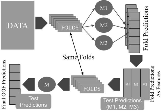
堆叠不是什么高深莫测的事。它很直接。如果你做了正确的交叉验证(cross-validation),并且在建模任务的整个过程中保持折不变,那么什么都不会过拟合。
让我用简单的要点来描述这个想法。
- 把训练数据分成若干折。
- 训练一组模型:M1, M2……Mn。
- 使用所有这些模型创建完整的训练预测(使用折外(out of fold)训练)和测试预测。
- 到目前为止这是第 1 层(Level - 1,L1)。
- 把这些模型的折预测作为特征用于另一个模型。这就是第 2 层(Level - 2,L2)模型。
- 使用和之前相同的折来训练这个 L2 模型。
- 现在在训练集和测试集上创建 OOF(折外,out of fold)预测。
- 现在你有了训练数据的 L2 预测,以及最终的测试集预测。
你可以不断重复 L1 部分,想创建多少层就创建多少层。
有时候,你还会遇到一个术语叫融合(blending)。如果遇到了,不用太担心。它无非就是用保留集(holdout set)代替多个折的堆叠。
必须指出的是,本章所描述的内容可以应用于任何类型的问题:分类(classification)、回归(regression)、多标签分类(multi-label classification)等等。