文本分类与回归

文本问题是我最喜欢的。一般来说，这类问题也被称为自然语言处理（Natural Language Processing，NLP）问题。NLP 问题与图像问题有一点相似：它们都很不一样。你需要构建一些你在表格数据问题中从未构建过的流水线（pipeline）。你需要理解业务场景，才能构建出好的模型。顺便说一句，这对机器学习中的任何事情都是成立的。构建模型能让你达到一定水平，但要想提升并为你要构建模型的业务做出贡献，你必须理解模型如何影响业务。我们在这里就不谈太多哲学了。

NLP 问题有很多种类型，最常见的是字符串的分类。很多时候，我们会看到有人在表格数据或图像上做得很好，但一遇到文本，他们甚至不知道从哪里开始。文本数据与其他类型的数据集并没有什么不同。对计算机来说，一切都是数字。

假设我们从情感分类（sentiment classification）这一基础任务开始。我们将尝试从电影评论中分类情感。所以，你有一段文本，它关联着一种情感。你会如何处理这类问题？直接上深度神经网络，对吧？或者布偶（muppets）会来拯救你？不，完全错了。你要从基础开始。先看看这些数据长什么样。

我们从 IMDB 电影评论数据集¹开始，它包含 25000 条正面情感评论和 25000 条负面情感评论。

我在这里讨论的概念几乎可以应用于任何文本分类数据集。

这个数据集很容易理解。一条评论对应一个目标变量。注意，我写的是评论（review）而不是句子（sentence）。一条评论是一堆句子的集合。所以，到目前为止你可能只见过对单个句子的分类，但在这个问题中，我们要对多个句子进行分类。简单来说，这意味着不只是单个句子贡献情感，情感分数是多个句子分数的组合。图 1 展示了该数据的一个快照。

图 1. IMDB 电影评论数据集的快照。

		评论情感
	0 One of the other reviewers has mentioned that …	positive
1	A wonderful little production. The…	positive
2	I thought this was a wonderful way to spend ti…	positive
3	Basically there’s a family where a little boy …	negative
4	Petter Mattei’s “Love in the Time of Money” is…	positive

你会如何着手解决这样的问题？

一个简单的办法是手工制作两个单词列表。一个列表包含你能想象到的所有正面词汇，例如 good、awesome、nice 等，另一个列表包含所有负面词汇，例如 bad、evil 等。负面词汇的例子我们就不举了，否则这本书就得只面向 18 岁以上读者了。一旦你有了这些列表，你甚至不需要模型就能做出预测。这些列表也被称为情感词典（sentiment lexicon）。互联网上有许多不同语言的情感词典。

你可以用一个简单的计数器，统计句子中正面和负面词汇的数量。如果正面词汇的数量更多，就是正面情感；如果负面词汇的数量更多，就是负面情感的句子。如果句子中两者都没有出现，你可以说这个句子是中性情感。这是最古老的方法之一，有些人至今仍在用。它也不需要太多代码。

def find_sentiment(sentence, pos, neg):
    """
    This function returns sentiment of sentence
    :param sentence: sentence, a string
    :param pos: set of positive words
    :param neg: set of negative words
    :return: returns positive, negative or neutral sentiment
    """
    # split sentence by a space
    # "this is a sentence!" becomes:
    # ["this", "is" "a", "sentence!"]
    # note that im splitting on all whitespaces
    # if you want to split by space use .split(" ")
    sentence = sentence.split()
    # make sentence into a set
    sentence = set(sentence)
    # check number of common words with positive
    num_common_pos = len(sentence.intersection(pos))
    # check number of common words with negative
    num_common_neg = len(sentence.intersection(neg))
    # make conditions and return
    # see how return used eliminates if else
    if num_common_pos > num_common_neg:
        return "positive"
    if num_common_pos < num_common_neg:
        return "negative"
    return "neutral"

然而，这种方法没有考虑太多因素。而且正如你所看到的，我们的 split() 也并非完美。如果你使用 split()，像这样的句子：

'hi, how are you?' gets split into ['hi,', 'how', 'are', 'you?']

这并不理想，因为你会看到逗号和问号没有被分开。因此，如果你的预处理没有在切分之前处理这些特殊字符，就不推荐使用这种方法。把字符串切分成单词列表被称为分词（tokenization）。最流行的分词工具之一来自 NLTK（Natural Language Tool Kit，自然语言工具包）。

In [X]: from nltk.tokenize import word_tokenize
In [X]: sentence = "hi, how are you?"

In [X]: sentence.split()
Out[X]: ['hi,', 'how', 'are', 'you?']

In [X]: word_tokenize(sentence)
Out[X]: ['hi', ',', 'how', 'are', 'you', '?']

正如你所看到的，使用 NLTK 的 word_tokenize 后，同一个句子的切分方式要好得多。用它来与单词列表做比较，效果也会好得多！这就是我们将应用到第一个情感检测模型上的方法。

在处理 NLP 分类问题时，你应该始终尝试的基础模型之一是词袋（bag of words）。在词袋中，我们创建一个巨大的稀疏矩阵（sparse matrix），存储语料库（corpus，即所有文档，也就是所有句子）中所有单词的计数。为此，我们将使用 scikit-learn 的 CountVectorizer。让我们看看它是如何工作的。

from sklearn.feature_extraction.text import CountVectorizer

# create a corpus of sentences
corpus = [
    "hello, how are you?",
    "im getting bored at home. And you? What do you think?",
    "did you know about counts",
    "let's see if this works!",
    "YES!!!!"
]

# initialize CountVectorizer
ctv = CountVectorizer()

# fit the vectorizer on corpus
ctv.fit(corpus)
corpus_transformed = ctv.transform(corpus)

如果我们打印 corpus_transformed，会得到类似下面的结果：

(0, 2) 1
(0, 9) 1
(0, 11) 1
(0, 22) 1
(1, 1) 1
(1, 3) 1
(1, 4) 1
(1, 7) 1
(1, 8) 1
(1, 10) 1
(1, 13) 1
(1, 17) 1
(1, 19) 1
(1, 22) 2
(2, 0) 1
(2, 5) 1
(2, 6) 1
(2, 14) 1
(2, 22) 1
(3, 12) 1
(3, 15) 1
(3, 16) 1
(3, 18) 1
(3, 20) 1
(4, 21) 1

我们在之前的章节中已经见过这种表示。它就是稀疏表示。因此，我们的语料库现在是一个稀疏矩阵，其中第一个样本有四个元素，第二个样本有十个元素，第三个样本有五个元素，依此类推。我们还看到这些元素都关联着一个计数。有些出现了两次，有些只出现一次。例如，在样本 2（第 1 行）中，我们看到第 22 列的值为 2。这是为什么呢？第 22 列又是什么呢？

CountVectorizer 的工作方式是：首先对句子进行分词，然后为每个词元（token）分配一个值。因此，每个词元都由一个唯一的索引表示。我们看到的这些列就是这些唯一索引。CountVectorizer 会存储这些信息。

print(ctv.vocabulary_)

{'hello': 9, 'how': 11, 'are': 2, 'you': 22, 'im': 13, 'getting': 8,
 'bored': 4, 'at': 3, 'home': 10, 'and': 1, 'what': 19, 'do': 7,
 'think': 17, 'did': 6, 'know': 14, 'about': 0, 'counts': 5,
 'let': 15, 'see': 16, 'if': 12, 'this': 18, 'works': 20, 'yes': 21}

我们看到索引 22 属于 ‘you’，而在第二个句子中 ‘you’ 出现了两次。所以计数是 2。我希望现在词袋是什么已经很清楚了。但我们漏掉了一些特殊字符。有时这些特殊字符也可能有用。例如，’?’ 在大多数句子中表示疑问。让我们把 scikit-learn 的 word_tokenize 集成到 CountVectorizer 中，看看会发生什么。

from sklearn.feature_extraction.text import CountVectorizer
from nltk.tokenize import word_tokenize

# create a corpus of sentences
corpus = [
    "hello, how are you?",
    "im getting bored at home. And you? What do you think?",
    "did you know about counts",
    "let's see if this works!",
    "YES!!!!"
]

# initialize CountVectorizer with word_tokenize from nltk
# as the tokenizer
ctv = CountVectorizer(tokenizer=word_tokenize, token_pattern=None)

# fit the vectorizer on corpus
ctv.fit(corpus)
corpus_transformed = ctv.transform(corpus)
print(ctv.vocabulary_)

这会把我们的词汇表变成：

{'hello': 14, ',': 2, 'how': 16, 'are': 7, 'you': 27, '?': 4, 'im': 18,
 'getting': 13, 'bored': 9, 'at': 8, 'home': 15, '.': 3, 'and': 6,
 'what': 24, 'do': 12, 'think': 22, 'did': 11, 'know': 19, 'about': 5,
 'counts': 10, 'let': 20, "'s": 1, 'see': 21, 'if': 17, 'this': 23,
 'works': 25, '!': 0, 'yes': 26}

现在，词汇表中的单词更多了。因此，我们现在可以用 IMDB 数据集中的所有句子创建一个稀疏矩阵，然后构建模型。这个数据集中正面和负面样本的比例是 1:1，因此我们可以使用准确率（accuracy）作为评估指标。我们将使用 StratifiedKFold，并编写一个脚本训练五折。你会问用什么模型？对于高维稀疏数据，最快的模型是什么？逻辑回归（logistic regression）。我们将先用逻辑回归处理这个数据集，建立我们的第一个真正的基准（benchmark）。

让我们看看怎么做。

# import what we need
import pandas as pd
from nltk.tokenize import word_tokenize
from sklearn import linear_model
from sklearn import metrics
from sklearn import model_selection
from sklearn.feature_extraction.text import CountVectorizer

if __name__ == "__main__":
    # read the training data
    df = pd.read_csv("../input/imdb.csv")

    # map positive to 1 and negative to 0
    df.sentiment = df.sentiment.apply(
        lambda x: 1 if x == "positive" else 0
    )

    # we create a new column called kfold and fill it with -1
    df["kfold"] = -1

    # the next step is to randomize the rows of the data
    df = df.sample(frac=1).reset_index(drop=True)

    # fetch labels
    y = df.sentiment.values

    # initiate the kfold class from model_selection module
    kf = model_selection.StratifiedKFold(n_splits=5)

    # fill the new kfold column
    for f, (t_, v_) in enumerate(kf.split(X=df, y=y)):
        df.loc[v_, 'kfold'] = f

    # we go over the folds created
    for fold_ in range(5):
        # temporary dataframes for train and test
        train_df = df[df.kfold != fold_].reset_index(drop=True)
        test_df = df[df.kfold == fold_].reset_index(drop=True)

        # initialize CountVectorizer with NLTK's word_tokenize
        # function as tokenizer
        count_vec = CountVectorizer(
            tokenizer=word_tokenize,
            token_pattern=None
        )

        # fit count_vec on training data reviews
        count_vec.fit(train_df.review)

        # transform training and validation data reviews
        xtrain = count_vec.transform(train_df.review)
        xtest = count_vec.transform(test_df.review)

        # initialize logistic regression model
        model = linear_model.LogisticRegression()

        # fit the model on training data reviews and sentiment
        model.fit(xtrain, train_df.sentiment)

        # make predictions on test data
        # threshold for predictions is 0.5
        preds = model.predict(xtest)

        # calculate accuracy
        accuracy = metrics.accuracy_score(test_df.sentiment, preds)

        print(f"Fold: {fold_}")
        print(f"Accuracy = {accuracy}")
        print("")

这段代码运行需要一些时间，但应该会给你以下输出：

❯ python ctv_logres.py
Fold: 0
Accuracy = 0.8903
Fold: 1
Accuracy = 0.897
Fold: 2
Accuracy = 0.891
Fold: 3
Accuracy = 0.8914
Fold: 4
Accuracy = 0.8931

哇，我们已经达到了 89% 的准确率，而我们所做的只是把词袋和逻辑回归结合使用！这太棒了！不过，这个模型训练花了很多时间，让我们看看用朴素贝叶斯（naïve Bayes）分类器能不能缩短时间。朴素贝叶斯分类器在 NLP 任务中相当流行，因为稀疏矩阵非常巨大，而朴素贝叶斯是一个简单的模型。要使用这个模型，我们只需要改一个 import 和模型那一行。让我们看看这个模型的表现。我们将使用 scikit-learn 的 MultinomialNB。

# import what we need
import pandas as pd
from nltk.tokenize import word_tokenize
from sklearn import naive_bayes
from sklearn import metrics
from sklearn import model_selection
from sklearn.feature_extraction.text import CountVectorizer
.
.
.
# initialize naive bayes model
model = naive_bayes.MultinomialNB()

# fit the model on training data reviews and sentiment
model.fit(xtrain, train_df.sentiment)
.
.

结果如下：

❯ python ctv_nb.py
Fold: 0
Accuracy = 0.8444
Fold: 1
Accuracy = 0.8499
Fold: 2
Accuracy = 0.8422
Fold: 3
Accuracy = 0.8443
Fold: 4
Accuracy = 0.8455

我们看到这个分数比较低。但朴素贝叶斯模型非常快。

NLP 中另一个如今大多数人不愿了解或懒得去了解的方法是 TF-IDF。TF 是词频（term frequency），IDF 是逆文档频率（inverse document frequency）。光看这些术语可能觉得很难，但看了 TF 和 IDF 的公式，一切就一目了然了。

\[ TF(t) = \frac{\text{词项 } t \text{ 在文档中出现的次数}}{\text{文档中的词项总数}} \]\[ IDF(t) = \log\left(\frac{\text{文档总数}}{\text{包含词项 } t \text{ 的文档数}}\right) \]

而词项 t 的 TF-IDF 定义为：

\[ TF\text{-}IDF(t) = TF(t) \times IDF(t) \]

与 scikit-learn 中的 CountVectorizer 类似，我们还有 TfidfVectorizer。让我们试试像使用 CountVectorizer 一样使用它。

from sklearn.feature_extraction.text import TfidfVectorizer
from nltk.tokenize import word_tokenize

# create a corpus of sentences
corpus = [
    "hello, how are you?",
    "im getting bored at home. And you? What do you think?",
    "did you know about counts",
    "let's see if this works!",
    "YES!!!!"
]

# initialize TfidfVectorizer with word_tokenize from nltk
# as the tokenizer
tfv = TfidfVectorizer(tokenizer=word_tokenize, token_pattern=None)

# fit the vectorizer on corpus
tfv.fit(corpus)
corpus_transformed = tfv.transform(corpus)
print(corpus_transformed)

这会给出以下输出：

(0, 27) 0.2965698850220162
(0, 16) 0.4428321995085722
(0, 14) 0.4428321995085722
(0, 7) 0.4428321995085722
(0, 4) 0.35727423026525224
(0, 2) 0.4428321995085722
(1, 27) 0.35299699146792735
(1, 24) 0.2635440111190765
(1, 22) 0.2635440111190765
(1, 18) 0.2635440111190765
(1, 15) 0.2635440111190765
(1, 13) 0.2635440111190765
(1, 12) 0.2635440111190765
(1, 9) 0.2635440111190765
(1, 8) 0.2635440111190765
(1, 6) 0.2635440111190765
(1, 4) 0.42525129752567803
(1, 3) 0.2635440111190765
(2, 27) 0.31752680284846835
(2, 19) 0.4741246485558491
(2, 11) 0.4741246485558491
(2, 10) 0.4741246485558491
(2, 5) 0.4741246485558491
(3, 25) 0.38775666010579296
(3, 23) 0.38775666010579296
(3, 21) 0.38775666010579296
(3, 20) 0.38775666010579296
(3, 17) 0.38775666010579296
(3, 1) 0.38775666010579296
(3, 0) 0.3128396318588854
(4, 26) 0.2959842226518677
(4, 0) 0.9551928286692534

我们看到，这次得到的不是整数值，而是浮点数。把 CountVectorizer 换成 TfidfVectorizer 也是小菜一碟。scikit-learn 还提供了 TfidfTransformer。如果你已经有了计数值，可以使用 TfidfTransformer，得到与 TfidfVectorizer 相同的行为。

# import what we need
import pandas as pd
from nltk.tokenize import word_tokenize
from sklearn import linear_model
from sklearn import metrics
from sklearn import model_selection
from sklearn.feature_extraction.text import TfidfVectorizer
.
.
# we go over the folds created
for fold_ in range(5):
    # temporary dataframes for train and test
    train_df = df[df.kfold != fold_].reset_index(drop=True)
    test_df = df[df.kfold == fold_].reset_index(drop=True)

    # initialize TfidfVectorizer with NLTK's word_tokenize
    # function as tokenizer
    tfidf_vec = TfidfVectorizer(
        tokenizer=word_tokenize,
        token_pattern=None
    )

    # fit tfidf_vec on training data reviews
    tfidf_vec.fit(train_df.review)

    # transform training and validation data reviews
    xtrain = tfidf_vec.transform(train_df.review)
    xtest = tfidf_vec.transform(test_df.review)

    # initialize logistic regression model
    model = linear_model.LogisticRegression()

    # fit the model on training data reviews and sentiment
    model.fit(xtrain, train_df.sentiment)

    # make predictions on test data
    # threshold for predictions is 0.5
    preds = model.predict(xtest)

    # calculate accuracy
    accuracy = metrics.accuracy_score(test_df.sentiment, preds)

    print(f"Fold: {fold_}")
    print(f"Accuracy = {accuracy}")
    print("")

看看 TF-IDF 与我们之前的逻辑回归模型在情感数据集上的表现会很有趣。

❯ python tfv_logres.py
Fold: 0
Accuracy = 0.8976
Fold: 1
Accuracy = 0.8998
Fold: 2
Accuracy = 0.8948
Fold: 3
Accuracy = 0.8912
Fold: 4
Accuracy = 0.8995

我们看到这些分数比 CountVectorizer 略高一些，因此它成了我们想要击败的新基准。

NLP 中另一个有趣的概念是 n-gram。N-gram 是按顺序组合的单词。N-gram 很容易创建。你只需要注意顺序。为了让事情更方便，我们可以使用 NLTK 的 n-gram 实现。

from nltk import ngrams
from nltk.tokenize import word_tokenize

# let's see 3 grams
N = 3

# input sentence
sentence = "hi, how are you?"

# tokenized sentence
tokenized_sentence = word_tokenize(sentence)

# generate n_grams
n_grams = list(ngrams(tokenized_sentence, N))
print(n_grams)

输出如下：

[('hi', ',', 'how'), (',', 'how', 'are'), ('how', 'are', 'you'), ('are', 'you', '?')]

类似地，我们也可以创建 2-gram、4-gram 等。现在，这些 n-gram 成为我们词汇表的一部分，当我们计算计数或 tf-idf 时，我们会把一个 n-gram 视为一个全新的词元。所以从某种意义上说，我们在一定程度上融入了上下文。scikit-learn 的 CountVectorizer 和 TfidfVectorizer 实现都通过 ngram_range 参数提供 n-gram 支持，该参数有最小值和最大值限制。默认是 (1, 1)。当我们把它改成 (1, 3) 时，我们就同时在考虑一元词（unigram）、二元词（bigram）和三元词（trigram）。代码改动很小。由于到目前为止 tf-idf 的结果最好，让我们看看把 n-gram 扩展到三元词会不会提升模型。

唯一需要改动的地方是 TfidfVectorizer 的初始化。

tfidf_vec = TfidfVectorizer(
    tokenizer=word_tokenize,
    token_pattern=None,
    ngram_range=(1, 3)
)

让我们看看是否有什么提升。

❯ python tfv_logres_trigram.py
Fold: 0
Accuracy = 0.8931
Fold: 1
Accuracy = 0.8941
Fold: 2
Accuracy = 0.897
Fold: 3
Accuracy = 0.8922
Fold: 4
Accuracy = 0.8847

看起来还行，但我们没有看到任何提升。也许只用二元词能带来提升。这部分我就不展示了。也许你可以自己试试。

NLP 基础中还有很多内容。有一个术语你必须了解：词干提取（stemming）。另一个是词形还原（lemmatization）。词干提取和词形还原都把单词化简为最小的形式。在词干提取中，处理后的单词被称为词干（stemmed word）；在词形还原中，它被称为词元（lemma）。必须指出的是，词形还原比词干提取更激进，而词干提取更流行、应用更广。词干提取和词形还原都来自语言学。如果你打算为某种语言制作词干提取器或词形还原器，你需要对该语言有深入的了解。详细讨论它们意味着给这本书再增加一章。使用 NLTK 包可以轻松完成词干提取和词形还原。让我们看一些两者的例子。词干提取器和词形还原器有很多种。我将用最常用的 Snowball Stemmer 和 WordNet Lemmatizer 来演示一个例子。

from nltk.stem import WordNetLemmatizer
from nltk.stem.snowball import SnowballStemmer

# initialize lemmatizer
lemmatizer = WordNetLemmatizer()

# initialize stemmer
stemmer = SnowballStemmer("english")

words = ["fishing", "fishes", "fished"]

for word in words:
    print(f"word={word}")
    print(f"stemmed_word={stemmer.stem(word)}")
    print(f"lemma={lemmatizer.lemmatize(word)}")
    print("")

这会打印：

word=fishing
stemmed_word=fish
lemma=fishing
word=fishes
stemmed_word=fish
lemma=fish
word=fished
stemmed_word=fish
lemma=fished

正如你所看到的，词干提取和词形还原彼此差异很大。当我们做词干提取时，得到的是一个单词的最小形式，它可能是也可能不是该单词所属语言词典中的词。然而，在词形还原的情况下，结果一定是一个词典中的词。你现在可以自己试试加入词干提取和词形还原，看看结果是否有所提升。

你应该了解的另一个主题是主题提取（topic extraction）。主题提取可以用非负矩阵分解（non-negative matrix factorization，NMF）或潜在语义分析（latent semantic analysis，LSA）来完成，后者也被广泛称为奇异值分解（singular value decomposition，SVD）。这些分解技术把数据降到给定数量的成分（component）。你可以把其中任何一种拟合到 CountVectorizer 或 TfidfVectorizer 得到的稀疏矩阵上。

让我们把它应用到之前用过的 TfidfVectorizer 上。

import pandas as pd
from nltk.tokenize import word_tokenize
from sklearn import decomposition
from sklearn.feature_extraction.text import TfidfVectorizer

# create a corpus of sentences
# we read only 10k samples from training data
# for this example
corpus = pd.read_csv("../input/imdb.csv", nrows=10000)
corpus = corpus.review.values

# initialize TfidfVectorizer with word_tokenize from nltk
# as the tokenizer
tfv = TfidfVectorizer(tokenizer=word_tokenize, token_pattern=None)

# fit the vectorizer on corpus
tfv.fit(corpus)

# transform the corpus using tfidf
corpus_transformed = tfv.transform(corpus)

# initialize SVD with 10 components
svd = decomposition.TruncatedSVD(n_components=10)

# fit SVD
corpus_svd = svd.fit(corpus_transformed)

# choose first sample and create a dictionary
# of feature names and their scores from svd
# you can change the sample_index variable to
# get dictionary for any other sample
sample_index = 0
feature_scores = dict(
    zip(
        tfv.get_feature_names(),
        corpus_svd.components_[sample_index]
    )
)

# once we have the dictionary, we can now
# sort it in decreasing order and get the
# top N topics
N = 5
print(sorted(feature_scores, key=feature_scores.get, reverse=True)[:N])

你可以用循环为多个样本运行它。

N = 5
for sample_index in range(5):
    feature_scores = dict(
        zip(
            tfv.get_feature_names(),
            corpus_svd.components_[sample_index]
        )
    )
    print(
        sorted(
            feature_scores,
            key=feature_scores.get,
            reverse=True
        )[:N]
    )

这给出以下输出。

['the', ',', '.', 'a', 'and']
['br', '<', '>', '/', '-']
['i', 'movie', '!', 'it', 'was']
[',', '!', "''", '``', 'you']
['!', 'the', '...', "''", '``']

你可以看到这完全没有什么意义。这种情况时有发生。那能怎么办呢？让我们试着做一下清洗，看看会不会变得有意义。

要清洗任何文本数据，尤其是当它在 pandas 数据框中时，你可以写一个函数。

import re
import string

def clean_text(s):
    """
    This function cleans the text a bit
    :param s: string
    :return: cleaned string
    """
    # split by all whitespaces
    s = s.split()

    # join tokens by single space
    # why we do this?
    # this will remove all kinds of weird space
    # "hi.   how are you" becomes
    # "hi. how are you"
    s = " ".join(s)

    # remove all punctuations using regex and string module
    s = re.sub(f'[{re.escape(string.punctuation)}]', '', s)

    # you can add more cleaning here if you want

    # and then return the cleaned string
    return s

这个函数会把像 ‘hi, how are you????’ 这样的字符串转换成 ‘hi how are you’。让我们把这个函数应用到之前的 SVD 代码上，看看它是否给提取出的主题带来价值。使用 pandas，你可以用 apply 函数把清洗代码"应用"到任何给定的列上。

import pandas as pd
.
corpus = pd.read_csv("../input/imdb.csv", nrows=10000)
corpus.loc[:, "review"] = corpus.review.apply(clean_text)
.
.

注意，我们只在主 SVD 脚本中添加了一行代码，这就是使用 pandas 函数和 apply 的美妙之处。这次生成的主题如下。

['the', 'a', 'and', 'of', 'to']
['i', 'movie', 'it', 'was', 'this']
['the', 'was', 'i', 'were', 'of']
['her', 'was', 'she', 'i', 'he']
['br', 'to', 'they', 'he', 'show']

呼！至少比之前的好一些。但是你知道吗？你还可以通过在清洗函数中移除停用词（stopword）让它变得更好。什么是停用词？就是每种语言中都存在的高频词。例如，在英语中，这些词是 ‘a’、‘an’、’the’、‘for’ 等。移除停用词并不总是一个明智的选择，这在很大程度上取决于业务问题。像 ‘I need a new dog’ 这样的句子在移除停用词后会变成 ’need new dog’，于是我们就不知道是谁需要一条新狗了。

如果我们总是移除停用词，会丢失大量上下文信息。你可以在 NLTK 中找到多种语言的停用词，如果没有，你也可以在你喜欢的搜索引擎上快速搜索找到。

让我们转向如今大多数人喜欢使用的方法：深度学习。但首先，我们必须知道什么是词嵌入（word embedding）。你已经看到，到目前为止我们把词元转换成了数字。因此，如果给定语料库中有 N 个唯一词元，它们可以用 0 到 N-1 的整数表示。现在我们将用向量来表示这些整数词元。这种把单词表示为向量的方式被称为词嵌入或词向量。谷歌的 Word2Vec 是把单词转换成向量的最古老的方法之一。我们还有 Facebook 的 FastText 和斯坦福的 GloVe（Global Vectors for Word Representation，用于词表示的全局向量）。这些方法彼此之间差异很大。

基本思路是构建一个浅层网络，通过重构输入句子来学习单词的嵌入。因此，你可以训练一个网络，利用周围的单词来预测一个缺失的单词，在这个过程中，网络会学习并更新所有相关单词的嵌入。这种方法也被称为连续词袋（Continuous Bag of Words，CBoW）模型。你也可以反过来，取一个单词来预测它的上下文单词。这被称为跳字（skip-gram）模型。Word2Vec 可以用这两种方法学习嵌入。

FastText 则学习字符 n-gram 的嵌入。就像单词 n-gram 一样，如果我们使用字符，它就被称为字符 n-gram；最后，GloVe 通过共现矩阵（co-occurrence matrix）来学习这些嵌入。所以，我们可以说所有这些不同类型的嵌入最终都返回一个字典，其中键是语料库（例如英语维基百科）中的一个单词，值是一个大小为 N（通常是 300）的向量。

图 1：在二维空间中可视化词嵌入。

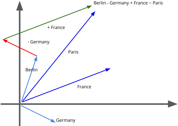
图 1 展示了二维空间中词嵌入的可视化。假设我们已经以某种方式把单词表示在了二维空间中。图 1 显示，如果你用柏林（德国的首都）的向量减去德国的向量，再加上法国的向量，你会得到一个接近巴黎（法国的首都）向量的向量。这表明嵌入也适用于类比推理。这并不总是成立的，但这样的例子有助于理解词嵌入的用处。像 ‘hi, how are you’ 这样的句子可以用一组向量表示如下。

hi	─>	[大小为 300 的向量 (v1)]
,	─>	[大小为 300 的向量 (v2)]
how	─>	[大小为 300 的向量 (v3)]
are	─>	[大小为 300 的向量 (v4)]
you	─>	[大小为 300 的向量 (v5)]
?	─>	[大小为 300 的向量 (v6)]

使用这些信息有多种方式。最简单的方式之一是按原样使用嵌入。正如你在上面的例子中看到的，每个单词都有一个 1x300 的嵌入向量。利用这些信息，我们可以计算整个句子的嵌入。有多种方法可以做到这一点。下面展示了其中一种方法。在这个函数中，我们取出给定句子中的所有单词向量，然后由这些词元的全部单词向量生成一个归一化词向量。这为我们提供了一个句向量（sentence vector）。

import numpy as np

def sentence_to_vec(s, embedding_dict, stop_words, tokenizer):
    """
    Given a sentence and other information, this function returns
    embedding for the whole sentence
    :param s: sentence, string
    :param embedding_dict: dictionary word:vector
    :param stop_words: list of stop words, if any
    :param tokenizer: a tokenization function
    """
    # convert sentence to string and lowercase it
    words = str(s).lower()

    # tokenize the sentence
    words = tokenizer(words)

    # remove stop word tokens
    words = [w for w in words if not w in stop_words]

    # keep only alpha-numeric tokens
    words = [w for w in words if w.isalpha()]

    # initialize empty list to store embeddings
    M = []
    for w in words:
        # for every word, fetch the embedding from
        # the dictionary and append to list of
        # embeddings
        if w in embedding_dict:
            M.append(embedding_dict[w])

    # if we dont have any vectors, return zeros
    if len(M) == 0:
        return np.zeros(300)

    # convert list of embeddings to array
    M = np.array(M)

    # calculate sum over axis=0
    v = M.sum(axis=0)

    # return normalized vector
    return v / np.sqrt((v ** 2).sum())

我们可以用这种方法把所有样本转换成一个向量。我们能用 fastText 向量来提升之前的结果吗？每条评论我们都有 300 个特征。

# fasttext.py
import io
import numpy as np
import pandas as pd
from nltk.tokenize import word_tokenize
from sklearn import linear_model
from sklearn import metrics
from sklearn import model_selection
from sklearn.feature_extraction.text import TfidfVectorizer


def load_vectors(fname):
    # taken from: https://fasttext.cc/docs/en/english-vectors.html
    fin = io.open(
        fname,
        'r',
        encoding='utf-8',
        newline='\n',
        errors='ignore'
    )
    n, d = map(int, fin.readline().split())
    data = {}
    for line in fin:
        tokens = line.rstrip().split(' ')
        data[tokens[0]] = list(map(float, tokens[1:]))
    return data


def sentence_to_vec(s, embedding_dict, stop_words, tokenizer):
    .
    .

if __name__ == "__main__":
    # read the training data
    df = pd.read_csv("../input/imdb.csv")

    # map positive to 1 and negative to 0
    df.sentiment = df.sentiment.apply(
        lambda x: 1 if x == "positive" else 0
    )

    # the next step is to randomize the rows of the data
    df = df.sample(frac=1).reset_index(drop=True)

    # load embeddings into memory
    print("Loading embeddings")
    embeddings = load_vectors("../input/crawl-300d-2M.vec")

    # create sentence embeddings
    print("Creating sentence vectors")
    vectors = []
    for review in df.review.values:
        vectors.append(
            sentence_to_vec(
                s=review,
                embedding_dict=embeddings,
                stop_words=[],
                tokenizer=word_tokenize
            )
        )
    vectors = np.array(vectors)

    # fetch labels
    y = df.sentiment.values

    # initiate the kfold class from model_selection module
    kf = model_selection.StratifiedKFold(n_splits=5)

    # fill the new kfold column
    for fold_, (t_, v_) in enumerate(kf.split(X=vectors, y=y)):
        print(f"Training fold: {fold_}")

        # temporary dataframes for train and test
        xtrain = vectors[t_, :]
        ytrain = y[t_]
        xtest = vectors[v_, :]
        ytest = y[v_]

        # initialize logistic regression model
        model = linear_model.LogisticRegression()

        # fit the model on training data reviews and sentiment
        model.fit(xtrain, ytrain)

        # make predictions on test data
        # threshold for predictions is 0.5
        preds = model.predict(xtest)

        # calculate accuracy
        accuracy = metrics.accuracy_score(ytest, preds)

        print(f"Accuracy = {accuracy}")
        print("")

这给出以下结果。

❯ python fasttext.py
Loading embeddings
Creating sentence vectors
Training fold: 0
Accuracy = 0.8619
Training fold: 1
Accuracy = 0.8661
Training fold: 2
Accuracy = 0.8544
Training fold: 3
Accuracy = 0.8624
Training fold: 4
Accuracy = 0.8595

哇！这相当出人意料。我们得到了很棒的结果，而我们所做的只是使用 FastText 嵌入。试着把嵌入换成 GloVe，看看会发生什么。我把它留作你的练习。

当我们谈论文本数据时，我们必须牢记一件事。文本数据与时间序列数据非常相似。我们评论中的任何样本都是一系列不同时间戳上的词元序列，时间戳按递增顺序排列，每个词元都可以表示为一个向量/嵌入，如图 2 所示。

图 2：把词元表示为嵌入，并将其视为时间序列

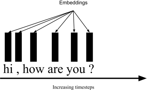
这意味着我们可以使用广泛用于时间序列数据的模型，比如长短期记忆网络（Long Short Term Memory，LSTM）、门控循环单元（Gated Recurrent Units，GRU），甚至卷积神经网络（Convolutional Neural Networks，CNN）。让我们看看如何在这个数据集上训练一个简单的双向 LSTM（bidirectional LSTM）模型。

首先，我们将创建一个项目。项目名随你取。然后我们的第一步是划分数据用于交叉验证。

# create_folds.py
# import pandas and model_selection module of scikit-learn
import pandas as pd
from sklearn import model_selection

if __name__ == "__main__":
    # Read training data
    df = pd.read_csv("../input/imdb.csv")

    # map positive to 1 and negative to 0
    df.sentiment = df.sentiment.apply(
        lambda x: 1 if x == "positive" else 0
    )

    # we create a new column called kfold and fill it with -1
    df["kfold"] = -1

    # the next step is to randomize the rows of the data
    df = df.sample(frac=1).reset_index(drop=True)

    # fetch labels
    y = df.sentiment.values

    # initiate the kfold class from model_selection module
    kf = model_selection.StratifiedKFold(n_splits=5)

    # fill the new kfold column
    for f, (t_, v_) in enumerate(kf.split(X=df, y=y)):
        df.loc[v_, 'kfold'] = f

    # save the new csv with kfold column
    df.to_csv("../input/imdb_folds.csv", index=False)

一旦我们把数据集划分成折（fold），就在 dataset.py 中创建一个简单的数据集类。Dataset 类返回训练或验证数据的一个样本。

# dataset.py
import torch

class IMDBDataset:
    def __init__(self, reviews, targets):
        """
        :param reviews: this is a numpy array
        :param targets: a vector, numpy array
        """
        self.reviews = reviews
        self.target = targets

    def __len__(self):
        # returns length of the dataset
        return len(self.reviews)

    def __getitem__(self, item):
        # for any given item, which is an int,
        # return review and targets as torch tensor
        # item is the index of the item in concern
        review = self.reviews[item, :]
        target = self.target[item]

        return {
            "review": torch.tensor(review, dtype=torch.long),
            "target": torch.tensor(target, dtype=torch.float)
        }

数据集类完成后，我们可以创建 lstm.py，它包含我们的 LSTM 模型。

# lstm.py
import torch
import torch.nn as nn

class LSTM(nn.Module):
    def __init__(self, embedding_matrix):
        """
        :param embedding_matrix: numpy array with vectors for all words
        """
        super(LSTM, self).__init__()

        # number of words = number of rows in embedding matrix
        num_words = embedding_matrix.shape[0]

        # dimension of embedding is num of columns in the matrix
        embed_dim = embedding_matrix.shape[1]

        # we define an input embedding layer
        self.embedding = nn.Embedding(
            num_embeddings=num_words,
            embedding_dim=embed_dim
        )

        # embedding matrix is used as weights of
        # the embedding layer
        self.embedding.weight = nn.Parameter(
            torch.tensor(
                embedding_matrix,
                dtype=torch.float32
            )
        )

        # we dont want to train the pretrained embeddings
        self.embedding.weight.requires_grad = False

        # a simple bidirectional LSTM with
        # hidden size of 128
        self.lstm = nn.LSTM(
            embed_dim,
            128,
            bidirectional=True,
            batch_first=True,
        )

        # output layer which is a linear layer
        # we have only one output
        # input (512) = 128 + 128 for mean and same for max pooling
        self.out = nn.Linear(512, 1)

    def forward(self, x):
        # pass data through embedding layer
        # the input is just the tokens
        x = self.embedding(x)

        # move embedding output to lstm
        x, _ = self.lstm(x)

        # apply mean and max pooling on lstm output
        avg_pool = torch.mean(x, 1)
        max_pool, _ = torch.max(x, 1)

        # concatenate mean and max pooling
        # this is why size is 512
        # 128 for each direction = 256
        # avg_pool = 256 and max_pool = 256
        out = torch.cat((avg_pool, max_pool), 1)

        # pass through the output layer and return the output
        out = self.out(out)

        # return linear output
        return out

现在，我们创建 engine.py，它包含我们的训练和评估函数。

# engine.py
import torch
import torch.nn as nn


def train(data_loader, model, optimizer, device):
    """
    This is the main training function that trains model for one epoch
    :param data_loader: this is the torch dataloader
    :param model: model (lstm model)
    :param optimizer: torch optimizer, e.g. adam, sgd, etc.
    :param device: this can be "cuda" or "cpu"
    """
    # set model to training mode
    model.train()

    # go through batches of data in data loader
    for data in data_loader:
        # fetch review and target from the dict
        reviews = data["review"]
        targets = data["target"]

        # move the data to device that we want to use
        reviews = reviews.to(device, dtype=torch.long)
        targets = targets.to(device, dtype=torch.float)

        # clear the gradients
        optimizer.zero_grad()

        # make predictions from the model
        predictions = model(reviews)

        # calculate the loss
        loss = nn.BCEWithLogitsLoss()(
            predictions,
            targets.view(-1, 1)
        )

        # compute gradient of loss w.r.t.
        # all parameters of the model that are trainable
        loss.backward()

        # single optimization step
        optimizer.step()


def evaluate(data_loader, model, device):
    # initialize empty lists to store predictions
    # and targets
    final_predictions = []
    final_targets = []

    # put the model in eval mode
    model.eval()

    # disable gradient calculation
    with torch.no_grad():
        for data in data_loader:
            reviews = data["review"]
            targets = data["target"]

            reviews = reviews.to(device, dtype=torch.long)
            targets = targets.to(device, dtype=torch.float)

            # make predictions
            predictions = model(reviews)

            # move predictions and targets to list
            # we need to move predictions and targets to cpu too
            predictions = predictions.cpu().numpy().tolist()
            targets = data["target"].cpu().numpy().tolist()

            final_predictions.extend(predictions)
            final_targets.extend(targets)

    # return final predictions and targets
    return final_predictions, final_targets

这些函数将在 train.py 中帮助我们，train.py 用于训练多个折。

# train.py
import io
import torch
import numpy as np
import pandas as pd

# yes, we use tensorflow
# but not for training the model!
import tensorflow as tf
from sklearn import metrics
import config
import dataset
import engine
import lstm


def load_vectors(fname):
    # taken from: https://fasttext.cc/docs/en/english-vectors.html
    fin = io.open(
        fname,
        'r',
        encoding='utf-8',
        newline='\n',
        errors='ignore'
    )
    n, d = map(int, fin.readline().split())
    data = {}
    for line in fin:
        tokens = line.rstrip().split(' ')
        data[tokens[0]] = list(map(float, tokens[1:]))
    return data


def create_embedding_matrix(word_index, embedding_dict):
    """
    This function creates the embedding matrix.
    :param word_index: a dictionary with word:index_value
    :param embedding_dict: a dictionary with word:embedding_vector
    :return: a numpy array with embedding vectors for all known words
    """
    # initialize matrix with zeros
    embedding_matrix = np.zeros((len(word_index) + 1, 300))

    # loop over all the words
    for word, i in word_index.items():
        # if word is found in pre-trained embeddings,
        # update the matrix. if the word is not found,
        # the vector is zeros!
        if word in embedding_dict:
            embedding_matrix[i] = embedding_dict[word]

    # return embedding matrix
    return embedding_matrix


def run(df, fold):
    """
    Run training and validation for a given fold and dataset
    :param df: pandas dataframe with kfold column
    :param fold: current fold, int
    """
    # fetch training dataframe
    train_df = df[df.kfold != fold].reset_index(drop=True)

    # fetch validation dataframe
    valid_df = df[df.kfold == fold].reset_index(drop=True)

    print("Fitting tokenizer")
    # we use tf.keras for tokenization
    # you can use your own tokenizer and then you can
    # get rid of tensorflow
    tokenizer = tf.keras.preprocessing.text.Tokenizer()
    tokenizer.fit_on_texts(df.review.values.tolist())

    # convert training data to sequences
    # for example : "bad movie" gets converted to
    # [24, 27] where 24 is the index for bad and 27 is the
    # index for movie
    xtrain = tokenizer.texts_to_sequences(train_df.review.values)

    # similarly convert validation data to
    # sequences
    xtest = tokenizer.texts_to_sequences(valid_df.review.values)

    # zero pad the training sequences given the maximum length
    # this padding is done on left hand side
    # if sequence is > MAX_LEN, it is truncated on left hand side too
    xtrain = tf.keras.preprocessing.sequence.pad_sequences(
        xtrain,
        maxlen=config.MAX_LEN
    )

    # zero pad the validation sequences
    xtest = tf.keras.preprocessing.sequence.pad_sequences(
        xtest,
        maxlen=config.MAX_LEN
    )

    # initialize dataset class for training
    train_dataset = dataset.IMDBDataset(
        reviews=xtrain,
        targets=train_df.sentiment.values
    )

    # create torch dataloader for training
    # torch dataloader loads the data using dataset
    # class in batches specified by batch size
    train_data_loader = torch.utils.data.DataLoader(
        train_dataset,
        batch_size=config.TRAIN_BATCH_SIZE,
        num_workers=2
    )

    # initialize dataset class for validation
    valid_dataset = dataset.IMDBDataset(
        reviews=xtest,
        targets=valid_df.sentiment.values
    )

    # create torch dataloader for validation
    valid_data_loader = torch.utils.data.DataLoader(
        valid_dataset,
        batch_size=config.VALID_BATCH_SIZE,
        num_workers=1
    )

    print("Loading embeddings")
    # load embeddings as shown previously
    embedding_dict = load_vectors("../input/crawl-300d-2M.vec")
    embedding_matrix = create_embedding_matrix(
        tokenizer.word_index,
        embedding_dict
    )

    # create torch device, since we use gpu, we are using cuda
    device = torch.device("cuda")

    # fetch our LSTM model
    model = lstm.LSTM(embedding_matrix)

    # send model to device
    model.to(device)

    # initialize Adam optimizer
    optimizer = torch.optim.Adam(model.parameters(), lr=1e-3)

    print("Training Model")
    # set best accuracy to zero
    best_accuracy = 0

    # set early stopping counter to zero
    early_stopping_counter = 0

    # train and validate for all epochs
    for epoch in range(config.EPOCHS):
        # train one epoch
        engine.train(train_data_loader, model, optimizer, device)

        # validate
        outputs, targets = engine.evaluate(
            valid_data_loader,
            model,
            device
        )

        # use threshold of 0.5
        # please note we are using linear layer and no sigmoid
        # you should do this 0.5 threshold after sigmoid
        outputs = np.array(outputs) >= 0.5

        # calculate accuracy
        accuracy = metrics.accuracy_score(targets, outputs)

        print(
            f"FOLD:{fold}, Epoch: {epoch}, Accuracy Score = {accuracy}"
        )

        # simple early stopping
        if accuracy > best_accuracy:
            best_accuracy = accuracy
        else:
            early_stopping_counter += 1
            if early_stopping_counter > 2:
                break


if __name__ == "__main__":
    # load data
    df = pd.read_csv("../input/imdb_folds.csv")

    # train for all folds
    run(df, fold=0)
    run(df, fold=1)
    run(df, fold=2)
    run(df, fold=3)
    run(df, fold=4)

最后，我们还有 config.py。

# config.py
# we define all the configuration here
MAX_LEN = 128
TRAIN_BATCH_SIZE = 16
VALID_BATCH_SIZE = 8
EPOCHS = 10

让我们看看这能给我们带来什么。

❯ python train.py
FOLD:0, Epoch: 3, Accuracy Score = 0.9015
FOLD:1, Epoch: 4, Accuracy Score = 0.9007
FOLD:2, Epoch: 3, Accuracy Score = 0.8924
FOLD:3, Epoch: 2, Accuracy Score = 0.9
FOLD:4, Epoch: 1, Accuracy Score = 0.878

这是迄今为止我们得到的最好成绩。请注意，我只展示了每个折中准确率最好的轮次（epoch）。

你一定注意到了，我们使用了预训练嵌入和一个简单的双向 LSTM。如果你想更换模型，只需修改 lstm.py 中的模型，其他一切保持不变。这类代码做实验时只需要极少的改动，而且易于理解。例如，你可以自己学习嵌入而不是使用预训练嵌入，你可以使用其他预训练嵌入，你可以组合多个预训练嵌入，你可以使用 GRU，你可以在嵌入之后使用空间 dropout（spatial dropout），你可以在 LSTM 之后加一层 GRU，你可以加两层 LSTM，你可以采用 LSTM-GRU-LSTM 结构，你可以把 LSTM 换成卷积层，等等，而不需要对代码做太多修改。我提到的大部分内容只需要改动模型类。

当你使用预训练嵌入时，试着看看有多少单词找不到对应的嵌入，以及为什么。你有预训练嵌入的单词越多，结果就越好。我给你展示下面这个没有注释（！）的函数，你可以用它为任何与 glove 或 fastText 格式相同的预训练嵌入创建嵌入矩阵（可能需要一些修改）。

def load_embeddings(word_index, embedding_file, vector_length=300):
    """
    A general function to create embedding matrix
    :param word_index: word:index dictionary
    :param embedding_file: path to embeddings file
    :param vector_length: length of vector
    """
    max_features = len(word_index) + 1
    words_to_find = list(word_index.keys())
    more_words_to_find = []

    for wtf in words_to_find:
        more_words_to_find.append(wtf)
        more_words_to_find.append(str(wtf).capitalize())

    more_words_to_find = set(more_words_to_find)

    def get_coefs(word, *arr):
        return word, np.asarray(arr, dtype='float32')

    embeddings_index = dict(
        get_coefs(*o.strip().split(" "))
        for o in open(embedding_file)
        if o.split(" ")[0] in more_words_to_find
        and len(o) > 100
    )

    embedding_matrix = np.zeros((max_features, vector_length))

    for word, i in word_index.items():
        if i >= max_features:
            continue

        embedding_vector = embeddings_index.get(word)

        if embedding_vector is None:
            embedding_vector = embeddings_index.get(
                str(word).capitalize()
            )

        if embedding_vector is None:
            embedding_vector = embeddings_index.get(
                str(word).upper()
            )

        if (
            embedding_vector is not None
            and len(embedding_vector) == vector_length
        ):
            embedding_matrix[i] = embedding_vector

    return embedding_matrix

阅读并运行上面的函数，看看会发生什么。这个函数也可以修改为使用词干化或词形还原后的单词。最终，你希望训练语料库中未知单词的数量最少。另一个技巧是让嵌入层可训练，也就是把它设为可训练，然后训练网络。

到目前为止，我们已经为一个分类问题构建了很多模型。然而，现在是布偶的时代，越来越多的人正在转向基于 Transformer 的模型。基于 Transformer 的网络能够处理长距离的依赖关系。LSTM 只有在看过前一个单词之后才会看下一个单词。Transformer 则不是这样。它可以同时看到整个句子中的所有单词。因此，它还有一个优点：易于并行化，能更高效地利用 GPU。

Transformer 是一个非常宽泛的话题，模型太多了：BERT、RoBERTa、XLNet、XLM-RoBERTa、T5 等。我将展示一个通用方法，你可以用它处理我们一直在讨论的分类问题，适用于所有这些模型（T5 除外）。请注意，这些 Transformer 对训练所需的计算能力非常贪婪。因此，如果你没有高端的系统，训练一个模型可能需要比基于 LSTM 或 TF-IDF 的模型长得多的训练时间。

我们要做的第一件事是创建一个配置文件。

# config.py
import transformers

# this is the maximum number of tokens in the sentence
MAX_LEN = 512

# batch sizes is small because model is huge!
TRAIN_BATCH_SIZE = 8
VALID_BATCH_SIZE = 4

# let's train for a maximum of 10 epochs
EPOCHS = 10

# define path to BERT model files
BERT_PATH = "../input/bert_base_uncased/"

# this is where you want to save the model
MODEL_PATH = "model.bin"

# training file
TRAINING_FILE = "../input/imdb.csv"

# define the tokenizer
# we use tokenizer and model
# from huggingface's transformers
TOKENIZER = transformers.BertTokenizer.from_pretrained(
    BERT_PATH,
    do_lower_case=True
)

这里的配置文件是我们定义分词器和其他我们想频繁修改的参数的唯一地方——这样我们就可以做很多实验而不需要大量改动。

下一步是构建数据集类。

# dataset.py
import config
import torch

class BERTDataset:
    def __init__(self, review, target):
        """
        :param review: list or numpy array of strings
        :param targets: list or numpy array which is binary
        """
        self.review = review
        self.target = target

        # we fetch max len and tokenizer from config.py
        self.tokenizer = config.TOKENIZER
        self.max_len = config.MAX_LEN

    def __len__(self):
        # this returns the length of dataset
        return len(self.review)

    def __getitem__(self, item):
        # for a given item index, return a dictionary
        # of inputs
        review = str(self.review[item])
        review = " ".join(review.split())

        # encode_plus comes from hugginface's transformers
        # and exists for all tokenizers they offer
        # it can be used to convert a given string
        # to ids, mask and token type ids which are
        # needed for models like BERT
        # here, review is a string
        inputs = self.tokenizer.encode_plus(
            review,
            None,
            add_special_tokens=True,
            max_length=self.max_len,
            pad_to_max_length=True,
        )

        # ids are ids of tokens generated
        # after tokenizing reviews
        ids = inputs["input_ids"]

        # mask is 1 where we have input
        # and 0 where we have padding
        mask = inputs["attention_mask"]

        # token type ids behave the same way as
        # mask in this specific case
        # in case of two sentences, this is 0
        # for first sentence and 1 for second sentence
        token_type_ids = inputs["token_type_ids"]

        # now we return everything
        # note that ids, mask and token_type_ids
        # are all long datatypes and targets is float
        return {
            "ids": torch.tensor(
                ids,
                dtype=torch.long
            ),
            "mask": torch.tensor(
                mask,
                dtype=torch.long
            ),
            "token_type_ids": torch.tensor(
                token_type_ids,
                dtype=torch.long
            ),
            "targets": torch.tensor(
                self.target[item],
                dtype=torch.float
            )
        }

现在到了项目的核心，也就是模型。

# model.py
import config
import transformers
import torch.nn as nn

class BERTBaseUncased(nn.Module):
    def __init__(self):
        super(BERTBaseUncased, self).__init__()

        # we fetch the model from the BERT_PATH defined in
        # config.py
        self.bert = transformers.BertModel.from_pretrained(
            config.BERT_PATH
        )

        # add a dropout for regularization
        self.bert_drop = nn.Dropout(0.3)

        # a simple linear layer for output
        # yes, there is only one output
        self.out = nn.Linear(768, 1)

    def forward(self, ids, mask, token_type_ids):
        # BERT in its default settings returns two outputs
        # last hidden state and output of bert pooler layer
        # we use the output of the pooler which is of the size
        # (batch_size, hidden_size)
        # hidden size can be 768 or 1024 depending on
        # if we are using bert base or large respectively
        # in our case, it is 768
        # note that this model is pretty simple
        # you might want to use last hidden state
        # or several hidden states
        _, o2 = self.bert(
            ids,
            attention_mask=mask,
            token_type_ids=token_type_ids
        )

        # pass through dropout layer
        bo = self.bert_drop(o2)

        # pass through linear layer
        output = self.out(bo)

        # return output
        return output

这个模型返回单个输出。我们可以使用带 logits 的二元交叉熵损失（binary cross-entropy loss），它先应用 sigmoid，然后计算损失。这在 engine.py 中完成。

# engine.py
import torch
import torch.nn as nn


def loss_fn(outputs, targets):
    """
    This function returns the loss.
    :param outputs: output from the model (real numbers)
    :param targets: input targets (binary)
    """
    return nn.BCEWithLogitsLoss()(outputs, targets.view(-1, 1))


def train_fn(data_loader, model, optimizer, device, scheduler):
    """
    This is the training function which trains for one epoch
    :param data_loader: it is the torch dataloader object
    :param model: torch model, bert in our case
    :param optimizer: adam, sgd, etc
    :param device: can be cpu or cuda
    :param scheduler: learning rate scheduler
    """
    # put the model in training mode
    model.train()

    # loop over all batches
    for d in data_loader:
        # extract ids, token type ids and mask
        # from current batch
        # also extract targets
        ids = d["ids"]
        token_type_ids = d["token_type_ids"]
        mask = d["mask"]
        targets = d["targets"]

        # move everything to specified device
        ids = ids.to(device, dtype=torch.long)
        token_type_ids = token_type_ids.to(device, dtype=torch.long)
        mask = mask.to(device, dtype=torch.long)
        targets = targets.to(device, dtype=torch.float)

        # zero-grad the optimizer
        optimizer.zero_grad()

        # pass through the model
        outputs = model(
            ids=ids,
            mask=mask,
            token_type_ids=token_type_ids
        )

        # calculate loss
        loss = loss_fn(outputs, targets)

        # backward step the loss
        loss.backward()

        # step optimizer
        optimizer.step()

        # step scheduler
        scheduler.step()


def eval_fn(data_loader, model, device):
    """
    this is the validation function that generates predictions
    on validation data
    :param data_loader: it is the torch dataloader object
    :param model: torch model, bert in our case
    :param device: can be cpu or cuda
    :return: output and targets
    """
    # put model in eval mode
    model.eval()

    # initialize empty lists for
    # targets and outputs
    fin_targets = []
    fin_outputs = []

    # use the no_grad scope
    # its very important else you might
    # run out of gpu memory
    with torch.no_grad():
        # this part is same as training function
        # except for the fact that there is no
        # zero_grad of optimizer and there is no loss
        # calculation or scheduler steps.
        for d in data_loader:
            ids = d["ids"]
            token_type_ids = d["token_type_ids"]
            mask = d["mask"]
            targets = d["targets"]

            ids = ids.to(device, dtype=torch.long)
            token_type_ids = token_type_ids.to(device, dtype=torch.long)
            mask = mask.to(device, dtype=torch.long)
            targets = targets.to(device, dtype=torch.float)

            outputs = model(
                ids=ids,
                mask=mask,
                token_type_ids=token_type_ids
            )

            # convert targets to cpu and extend the final list
            targets = targets.cpu().detach()
            fin_targets.extend(targets.numpy().tolist())

            # convert outputs to cpu and extend the final list
            outputs = torch.sigmoid(outputs).cpu().detach()
            fin_outputs.extend(outputs.numpy().tolist())

    return fin_outputs, fin_targets

最后，我们准备好训练了。让我们看看训练脚本！

# train.py
import config
import dataset
import engine
import torch
import pandas as pd
import torch.nn as nn
import numpy as np
from model import BERTBaseUncased
from sklearn import model_selection
from sklearn import metrics
from transformers import AdamW
from transformers import get_linear_schedule_with_warmup


def train():
    # this function trains the model
    # read the training file and fill NaN values with "none"
    # you can also choose to drop NaN values in this
    # specific dataset
    dfx = pd.read_csv(config.TRAINING_FILE).fillna("none")

    # sentiment = 1 if its positive
    # else sentiment = 0
    dfx.sentiment = dfx.sentiment.apply(
        lambda x: 1 if x == "positive" else 0
    )

    # we split the data into single training
    # and validation fold
    df_train, df_valid = model_selection.train_test_split(
        dfx,
        test_size=0.1,
        random_state=42,
        stratify=dfx.sentiment.values
    )

    # reset index
    df_train = df_train.reset_index(drop=True)
    df_valid = df_valid.reset_index(drop=True)

    # initialize BERTDataset from dataset.py
    # for training dataset
    train_dataset = dataset.BERTDataset(
        review=df_train.review.values,
        target=df_train.sentiment.values
    )

    # create training dataloader
    train_data_loader = torch.utils.data.DataLoader(
        train_dataset,
        batch_size=config.TRAIN_BATCH_SIZE,
        num_workers=4
    )

    # initialize BERTDataset from dataset.py
    # for validation dataset
    valid_dataset = dataset.BERTDataset(
        review=df_valid.review.values,
        target=df_valid.sentiment.values
    )

    # create validation data loader
    valid_data_loader = torch.utils.data.DataLoader(
        valid_dataset,
        batch_size=config.VALID_BATCH_SIZE,
        num_workers=1
    )

    # initialize the cuda device
    # use cpu if you dont have GPU
    device = torch.device("cuda")

    # load model and send it to the device
    model = BERTBaseUncased()
    model.to(device)

    # create parameters we want to optimize
    # we generally dont use any decay for bias
    # and weight layers
    param_optimizer = list(model.named_parameters())
    no_decay = ["bias", "LayerNorm.bias", "LayerNorm.weight"]
    optimizer_parameters = [
        {
            "params": [
                p for n, p in param_optimizer
                if not any(nd in n for nd in no_decay)
            ],
            "weight_decay": 0.001,
        },
        {
            "params": [
                p for n, p in param_optimizer
                if any(nd in n for nd in no_decay)
            ],
            "weight_decay": 0.0,
        },
    ]

    # calculate the number of training steps
    # this is used by scheduler
    num_train_steps = int(
        len(df_train) / config.TRAIN_BATCH_SIZE * config.EPOCHS
    )

    # AdamW optimizer
    # AdamW is the most widely used optimizer
    # for transformer based networks
    optimizer = AdamW(optimizer_parameters, lr=3e-5)

    # fetch a scheduler
    # you can also try using reduce lr on plateau
    scheduler = get_linear_schedule_with_warmup(
        optimizer,
        num_warmup_steps=0,
        num_training_steps=num_train_steps
    )

    # if you have multiple GPUs
    # model model to DataParallel
    # to use multiple GPUs
    model = nn.DataParallel(model)

    # start training the epochs
    best_accuracy = 0
    for epoch in range(config.EPOCHS):
        engine.train_fn(
            train_data_loader,
            model,
            optimizer,
            device,
            scheduler
        )
        outputs, targets = engine.eval_fn(
            valid_data_loader,
            model,
            device
        )
        outputs = np.array(outputs) >= 0.5
        accuracy = metrics.accuracy_score(targets, outputs)
        print(f"Accuracy Score = {accuracy}")

        if accuracy > best_accuracy:
            torch.save(model.state_dict(), config.MODEL_PATH)
            best_accuracy = accuracy


if __name__ == "__main__":
    train()

乍一看可能很多，但一旦你理解了各个组成部分，其实并不多。你可以轻松地把它换成任何你想用的其他 Transformer 模型，只需要改动几行代码。

这个模型的准确率达到了 93%！哇！这比其他任何模型都好得多。但值得吗？

我们用 LSTM 就达到了 90%，而且 LSTM 简单得多、更容易训练、推理也更快。通过使用不同的数据处理或调整层数、节点数、dropout、学习率、更换优化器等参数，我们或许还能把那 90% 再提升一个百分点。这样一来，BERT 相比它只有约 2% 的收益。而另一方面，BERT 的训练时间要长得多，参数非常多，推理也很慢。归根结底，你应该看看自己的业务，做出明智的选择。不要仅仅因为 BERT 很"酷"就选择它。

必须指出的是，我们这里讨论的任务只是分类，但要把它改成回归、多标签或多分类，只需要改动几行代码。例如，同样的问题在多分类设定下会有多个输出和交叉熵（Cross-Entropy）损失。其他一切保持不变。自然语言处理非常庞大，我们只讨论了其中很小的一部分。不过从另一个角度看，这又是一大块内容，因为大多数工业模型都是分类或回归模型。如果我把所有细节都写出来，可能会写几百页，这就是为什么我决定把所有内容放在另一本书里：《Approaching (Almost) Any NLP Problem》（接近（几乎）任何 NLP 问题）！

Maas, Andrew L, Daly, Raymond E, Pham, Peter T, Huang, Dan, Ng, Andrew Y, and Potts, Christopher. Learning word vectors for sentiment analysis. In Proceedings of the 49th Annual Meeting of the Association for Computational Linguistics: Human Language Technologies-Volume 1, pp. 142-150. Association for Computational Linguistics, 2011. ↩︎