图像分类与分割
说到图像,过去几年里我们取得了大量成果。计算机视觉(computer vision)进展相当迅速,感觉计算机视觉的许多问题现在都容易解决多了。随着预训练模型(pretrained models)的出现和算力成本的下降,现在在家中训练一个接近最先进水平的模型,对于大多数与图像相关的问题来说简直是易如反掌。但图像问题有很多不同类型。你可以处理标准的二分类或多分类图像分类,也可以面对像自动驾驶汽车这样具有挑战性的问题。本书不会涉及自动驾驶汽车,但我们显然会处理一些最常见的图像问题。
我们可以对图像应用哪些不同的方法?图像不过是一个数字矩阵。计算机不能像人类那样看图像。它只看到数字,而图像就是这些数字。灰度图像(grayscale image)是一个二维矩阵,取值范围从 0 到 255。0 是黑色,255 是白色,中间是各种深浅的灰色。以前,在没有深度学习(deep learning)(或者说深度学习还不流行)的时候,人们会直接看像素(pixel)。每个像素就是一个特征。在 Python 中做这件事很容易:只需用 OpenCV 或 Python-PIL 读取灰度图像,转换为 numpy 数组,然后将矩阵展平(ravel)。如果你处理的是 RGB 图像,那么你有三个矩阵而不是一个,但思路是一样的。
import numpy as np
import matplotlib.pyplot as plt

# generate random numpy array with values from 0 to 255
# and a size of 256x256
random_image = np.random.randint(0, 256, (256, 256))

# initialize plot
plt.figure(figsize=(7, 7))

# show grayscale image, nb: cmap, vmin and vmax
plt.imshow(random_image, cmap='gray', vmin=0, vmax=255)
plt.show()
上面的代码使用 numpy 生成了一个随机矩阵。该矩阵的值范围为 0 到 255(含),大小为 256x256(也就是像素)。
图 1:二维图像数组(单通道)及其展平后的版本
| 图像 | 图像的展平版本 |
|---|
如你所见,展平后的版本不过是一个大小为 \(M\) 的向量,其中 \(M = N \times N\)。在本例中,这个向量的大小为 \(256 \times 256 = 65536\)。
现在,如果我们对数据集中的所有图像都这样做,每个样本就有 65536 个特征。我们可以很快地在这些数据上构建决策树(decision tree)模型、随机森林(random forest)或基于 SVM 的模型。这些模型会查看像素值,并尝试将正样本与负样本分开(在二分类(binary classification)问题的情况下)。
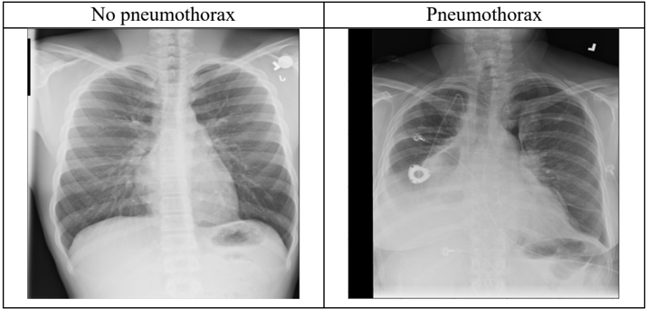
你们一定都听说过猫狗分类问题,这是一个经典问题。但让我们尝试点不一样的。如果你还记得,在评估指标那一章的开头,我向你介绍了气胸(pneumothorax)图像数据集。那么,让我们尝试构建一个模型来检测肺部 X 光图像是否存在气胸。也就是说,一个(并不那么)简单的二分类问题。
图 2:非气胸与气胸 X 光图像的对比 8。
8 https://www.kaggle.com/c/siim-acr-pneumothorax-segmentation
在图 2 中,你可以看到非气胸图像与气胸图像的对比。正如你可能已经注意到的,对于非专业人士(比如我)来说,甚至很难分辨出这些图像中哪些有气胸。
原始数据集的任务是检测气胸具体出现在哪里,但我们把问题改成了判断给定的 X 光图像是否存在气胸。别担心;我们会在本章中讲解"在哪里"的部分。该数据集包含 10675 张唯一图像,其中 2379 张有气胸(请注意,这些数字是在对数据做了一些清洗之后得到的,因此与原始数据集不完全一致)。正如数据医生会说的那样:这是一个典型的偏斜二分类(skewed binary classification)案例。因此,我们选择 AUC 作为评估指标,并采用分层 K 折交叉验证(stratified k-fold cross-validation)方案。
你可以把特征展平,然后尝试一些经典方法,如 SVM、RF 进行分类,这完全没问题,但它无法让你接近最先进的水平。此外,图像的大小是 1024x1024,在这个数据集上训练模型需要很长时间。不管怎样,让我们试着在这个数据上构建一个简单的随机森林模型。由于图像是灰度图,我们不需要做任何转换。我们将图像缩放到 256x256 以减小尺寸,并使用前面讨论过的 AUC 作为指标。
让我们看看它的表现如何。
import os
import numpy as np
import pandas as pd
from PIL import Image
from sklearn import ensemble
from sklearn import metrics
from sklearn import model_selection
from tqdm import tqdm


def create_dataset(training_df, image_dir):
    """
    This function takes the training dataframe and outputs training array and labels

    :param training_df: dataframe with ImageId, Target columns
    :param image_dir: location of images (folder), string
    :return: X, y (training array with features and labels)
    """
    # create empty list to store image vectors
    images = []

    # create empty list to store targets
    targets = []

    # loop over the dataframe
    for index, row in tqdm(
        training_df.iterrows(), total=len(training_df), desc="processing images"
    ):
        # get image id
        image_id = row["ImageId"]

        # create image path
        image_path = os.path.join(image_dir, image_id)

        # open image using PIL
        image = Image.open(image_path + ".png")

        # resize image to 256x256. we use bilinear resampling
        image = image.resize((256, 256), resample=Image.BILINEAR)

        # convert image to array
        image = np.array(image)

        # ravel
        image = image.ravel()

        # append images and targets lists
        images.append(image)
        targets.append(int(row["target"]))

    # convert list of list of images to numpy array
    images = np.array(images)

    # print size of this array
    print(images.shape)

    return images, targets


if __name__ == "__main__":
    csv_path = "/home/abhishek/workspace/siim_png/train.csv"
    image_path = "/home/abhishek/workspace/siim_png/train_png/"

    # read CSV with imageid and target columns
    df = pd.read_csv(csv_path)

    # we create a new column called kfold and fill it with -1
    df["kfold"] = -1

    # the next step is to randomize the rows of the data
    df = df.sample(frac=1).reset_index(drop=True)

    # fetch labels
    y = df.target.values

    # initiate the kfold class from model_selection module
    kf = model_selection.StratifiedKFold(n_splits=5)

    # fill the new kfold column
    for f, (t_, v_) in enumerate(kf.split(X=df, y=y)):
        df.loc[v_, "kfold"] = f

    # we go over the folds created
    for fold_ in range(5):
        # temporary dataframes for train and test
        train_df = df[df.kfold != fold_].reset_index(drop=True)
        test_df = df[df.kfold == fold_].reset_index(drop=True)

        # create train dataset
        # you can move this outside to save some computation time
        xtrain, ytrain = create_dataset(train_df, image_path)

        # create test dataset
        # you can move this outside to save some computation time
        xtest, ytest = create_dataset(test_df, image_path)

        # fit random forest without any modification of params
        clf = ensemble.RandomForestClassifier(n_jobs=-1)
        clf.fit(xtrain, ytrain)

        # predict probability of class 1
        preds = clf.predict_proba(xtest)[:, 1]

        # print results
        print(f"FOLD: {fold_}")
        print(f"AUC = {metrics.roc_auc_score(ytest, preds)}")
        print("")
这给出了大约 0.72 的平均 AUC。
这不算差,但希望我们能做得更好。你可以把这种方法用于图像,在过去的好时光里就是这样用的。SVM 在图像数据集上非常有名。深度学习已被证明是解决这类问题的最先进方法,因此我们接下来可以试试它。
我不会深入讲深度学习的历史以及谁发明了什么。相反,让我们看看最著名的深度学习模型之一 AlexNet,看看那里发生了什么。
图 3:AlexNet 架构 9。请注意,此图中的输入大小不是 224x224,而是 227x227。
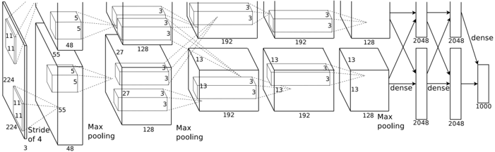
如今,你可能会说它是一个基础的深度卷积神经网络(deep convolutional neural network),但它是许多新深度网络(深度神经网络)的基础。我们看到图 3 中的网络是一个卷积神经网络(CNN),包含五个卷积层(convolution layer)、两个全连接层(dense layer)和一个输出层。我们还看到有最大池化(max pooling)。那是什么?让我们看看做深度学习时会遇到的一些术语。
图 4:大小为 8x8 的图像,滤波器大小为 3x3,步幅为 2。
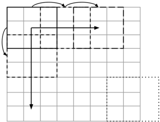
图 4 引入了两个新术语:滤波器(filter)和步幅(stride)。滤波器不过是二维矩阵,由给定的函数初始化。“He 初始化”,也就是"Kaiming 正态初始化",是卷积神经网络的一个不错选择。9 这是因为大多数现代网络使用 ReLU(Rectified Linear Units,线性整流单元)激活函数,而正确的初始化对于避免梯度消失(vanishing gradients)(即梯度趋近于零、网络权重不再变化)问题至关重要。这个滤波器与图像进行卷积(convolution)。卷积不过是滤波器与图像中当前重叠的像素之间的逐元素相乘(互相关)之和。你可以在任何高中数学教科书中读到更多关于卷积的内容。我们从图像的左上角开始对该滤波器进行卷积,然后水平移动它。如果每次移动 1 个像素,步幅就是 1;如果每次移动 2 个像素,步幅就是 2。这就是步幅的含义。
9 A. Krizhevsky, I. Sutskever, and G. Hinton. Imagenet classification with deep convolutional neural networks. In NIPS, 2012
步幅在自然语言处理中也是一个有用的概念,例如在问答系统中,当你需要从大型文本语料库中筛选出答案时。当水平方向移动完后,我们将滤波器以同样的步幅向下垂直移动,并重新从左边开始。图 4 还展示了一个超出图像边界的滤波器。在这种情况下,无法计算卷积,所以我们跳过它。如果你不想跳过,就需要对图像进行填充(padding)。还必须注意,卷积会减小图像的尺寸。填充也是保持图像尺寸不变的一种方法。在图 4 中,一个 3x3 的滤波器水平与垂直地移动,每次移动都会分别跳过两列和两行(即像素)。由于它跳过了两个像素,所以步幅 = 2。得到的图像尺寸是 \([(8-3) / 2] + 1 = 3.5\)。我们取 3.5 的向下取整,所以它是 3x3。你可以拿笔和纸手动移动滤波器来验证。
图 5:填充使我们能够获得与输入相同尺寸的图像
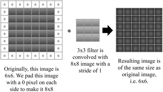
我们在图 5 中看到了填充的效果。现在,我们有一个 3x3 的滤波器,以步幅 1 移动。原始图像的大小是 6x6,我们添加了 1 的填充。填充为 1 意味着在每一侧各添加一次零像素来增大图像。在这种情况下,得到的图像将与输入图像大小相同,即 6x6。在处理深度神经网络时,你可能会遇到的另一个相关术语是膨胀(dilation),如图 6 所示。
图 6:膨胀的示例
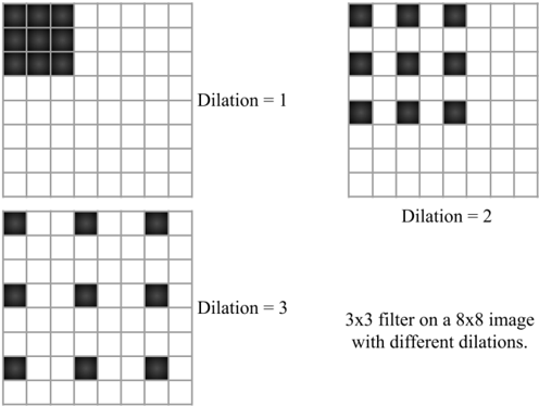
在膨胀中,我们按 \(N-1\) 扩展滤波器,其中 \(N\) 是膨胀率(dilation rate)的值,或简称为膨胀。在这种带膨胀的卷积核中,每次卷积都会跳过一些像素。这在分割任务中特别有效。请注意,我们只讨论了二维卷积。还有一维卷积,也有更高维度的卷积。它们都基于相同的基本概念。
接下来是最大池化。最大池化不过是一个返回最大值的滤波器。因此,与卷积不同,我们提取的是像素的最大值。类似地,平均池化(average pooling)或均值池化返回像素的均值。它们的使用方式与卷积核相同。池化比卷积更快,是一种对图像进行下采样(down-sample)的方式。最大池化能检测边缘,平均池化能平滑图像。
卷积神经网络和深度学习中的概念实在太多了。我讨论的是一些能帮助你入门的基础概念。现在,我们已经准备好开始用 PyTorch 构建我们的第一个卷积神经网络。PyTorch 提供了一种直观、简单的方式来实现深度神经网络,你不需要关心反向传播。我们在一个 Python 类中定义网络,并定义一个 forward 函数告诉 PyTorch 各层之间如何连接。在 PyTorch 中,图像的表示法是 BS、C、H、W,其中 BS 是批量大小(batch size),C 是通道(channel)数,H 是高度,W 是宽度。让我们看看 AlexNet 在 PyTorch 中是如何实现的。
import torch
import torch.nn as nn
import torch.nn.functional as F


class AlexNet(nn.Module):
    def __init__(self):
        super(AlexNet, self).__init__()
        # convolution part
        self.conv1 = nn.Conv2d(
            in_channels=3,
            out_channels=96,
            kernel_size=11,
            stride=4,
            padding=0,
        )
        self.pool1 = nn.MaxPool2d(kernel_size=3, stride=2)
        self.conv2 = nn.Conv2d(
            in_channels=96,
            out_channels=256,
            kernel_size=5,
            stride=1,
            padding=2,
        )
        self.pool2 = nn.MaxPool2d(kernel_size=3, stride=2)
        self.conv3 = nn.Conv2d(
            in_channels=256,
            out_channels=384,
            kernel_size=3,
            stride=1,
            padding=1,
        )
        self.conv4 = nn.Conv2d(
            in_channels=384,
            out_channels=384,
            kernel_size=3,
            stride=1,
            padding=1,
        )
        self.conv5 = nn.Conv2d(
            in_channels=384,
            out_channels=256,
            kernel_size=3,
            stride=1,
            padding=1,
        )
        self.pool3 = nn.MaxPool2d(kernel_size=3, stride=2)

        # dense part
        self.fc1 = nn.Linear(
            in_features=9216,
            out_features=4096,
        )
        self.dropout1 = nn.Dropout(0.5)
        self.fc2 = nn.Linear(
            in_features=4096,
            out_features=4096,
        )
        self.dropout2 = nn.Dropout(0.5)
        self.fc3 = nn.Linear(
            in_features=4096,
            out_features=1000,
        )

    def forward(self, image):
        # get the batch size, channels, height and width
        # of the input batch of images
        # original size: (bs, 3, 227, 227)
        bs, c, h, w = image.size()
        x = F.relu(self.conv1(image))  # size: (bs, 96, 55, 55)
        x = self.pool1(x)  # size: (bs, 96, 27, 27)
        x = F.relu(self.conv2(x))  # size: (bs, 256, 27, 27)
        x = self.pool2(x)  # size: (bs, 256, 13, 13)
        x = F.relu(self.conv3(x))  # size: (bs, 384, 13, 13)
        x = F.relu(self.conv4(x))  # size: (bs, 384, 13, 13)
        x = F.relu(self.conv5(x))  # size: (bs, 256, 13, 13)
        x = self.pool3(x)  # size: (bs, 256, 6, 6)
        x = x.view(bs, -1)  # size: (bs, 9216)
        x = F.relu(self.fc1(x))  # size: (bs, 4096)
        x = self.dropout1(x)  # size: (bs, 4096)
        # dropout does not change size
        # dropout is used for regularization
        # 0.3 dropout means that only 70% of the nodes
        # of the current layer are used for the next layer
        x = F.relu(self.fc2(x))  # size: (bs, 4096)
        x = self.dropout2(x)  # size: (bs, 4096)
        x = F.relu(self.fc3(x))  # size: (bs, 1000)
        # 1000 is number of classes in ImageNet Dataset
        # softmax is an activation function that converts
        # linear output to probabilities that add up to 1
        # for each sample in the batch
        x = torch.softmax(x, axis=1)  # size: (bs, 1000)
        return x
当你有一张 3x227x227 的图像,并应用大小为 11x11 的卷积滤波器时,这意味着你在应用一个大小为 11x11x3 的滤波器,并与大小为 227x227x3 的图像进行卷积。所以,现在你需要用三维而不是二维来思考。输出通道的数量就是独立应用于图像的、大小相同的不同卷积滤波器的数量。所以,在第一个卷积层中,输入通道是 3,也就是原始输入,即 R、G、B 三个通道。PyTorch 的 torchvision 提供了许多不同的模型,如 AlexNet,但必须注意,这个 AlexNet 实现与 torchvision 的不一样。torchvision 的 AlexNet 实现是另一篇论文中修改过的 AlexNet:Krizhevsky, A. One weird trick for parallelizing convolutional neural networks. CoRR, abs/1404.5997, 2014。
你可以为你的任务设计自己的卷积神经网络,很多时候从自己设计开始是个好主意。让我们构建一个网络,把本章最开始的数据集中的图像分类为有气胸或没有气胸。但首先,让我们准备一些文件。第一步是创建一个折(folds)文件,即 train.csv,但增加一个 kfold 新列。我们将创建五个折。由于本书中我已经展示了如何为不同数据集做这件事,这部分我就跳过,留作你的练习。对于基于 PyTorch 的神经网络,我们需要创建一个数据集类。数据集类的目标是返回一个数据项或样本。这个数据样本应包含训练或评估模型所需的一切。
# dataset.py
import torch
import numpy as np
from PIL import Image
from PIL import ImageFile

# sometimes, you will have images without an ending bit
# this takes care of those kind of (corrupt) images
ImageFile.LOAD_TRUNCATED_IMAGES = True


class ClassificationDataset:
    """
    A general classification dataset class that you can use
    for all kinds of image classification problems.
    For example, binary classification, multi-class, multi-label classification
    """

    def __init__(
        self,
        image_paths,
        targets,
        resize=None,
        augmentations=None,
    ):
        """
        :param image_paths: list of path to images
        :param targets: numpy array
        :param resize: tuple, e.g. (256, 256), resizes image if not None
        :param augmentations: albumentation augmentations
        """
        self.image_paths = image_paths
        self.targets = targets
        self.resize = resize
        self.augmentations = augmentations

    def __len__(self):
        """
        Return the total number of samples in the dataset
        """
        return len(self.image_paths)

    def __getitem__(self, item):
        """
        For a given "item" index, return everything we need to train a given model
        """
        # use PIL to open the image
        image = Image.open(self.image_paths[item])

        # convert image to RGB, we have single channel images
        image = image.convert("RGB")

        # grab correct targets
        targets = self.targets[item]

        # resize if needed
        if self.resize is not None:
            image = image.resize(
                (self.resize[1], self.resize[0]),
                resample=Image.BILINEAR,
            )

        # convert image to numpy array
        image = np.array(image)

        # if we have albumentation augmentations
        # add them to the image
        if self.augmentations is not None:
            augmented = self.augmentations(image=image)
            image = augmented["image"]

        # pytorch expects CHW instead of HWC
        image = np.transpose(image, (2, 0, 1)).astype(np.float32)

        # return tensors of image and targets
        # take a look at the types!
        # for regression tasks,
        # dtype of targets will change to torch.float
        return {
            "image": torch.tensor(image, dtype=torch.float),
            "targets": torch.tensor(targets, dtype=torch.long),
        }
现在我们还需要 engine.py。engine.py 包含训练和评估函数。让我们看看 engine.py 长什么样。
# engine.py
import torch
import torch.nn as nn
from tqdm import tqdm


def train(data_loader, model, optimizer, device):
    """
    This function does training for one epoch

    :param data_loader: this is the pytorch dataloader
    :param model: pytorch model
    :param optimizer: optimizer, for e.g. adam, sgd, etc
    :param device: cuda/cpu
    """
    # put the model in train mode
    model.train()

    # go over every batch of data in data loader
    for data in data_loader:
        # remember, we have image and targets
        # in our dataset class
        inputs = data["image"]
        targets = data["targets"]

        # move inputs/targets to cuda/cpu device
        inputs = inputs.to(device, dtype=torch.float)
        targets = targets.to(device, dtype=torch.float)

        # zero grad the optimizer
        optimizer.zero_grad()

        # do the forward step of model
        outputs = model(inputs)

        # calculate loss
        loss = nn.BCEWithLogitsLoss()(outputs, targets.view(-1, 1))

        # backward step the loss
        loss.backward()

        # step optimizer
        optimizer.step()

        # if you have a scheduler, you either need to
        # step it here or you have to step it after
        # the epoch. here, we are not using any learning
        # rate scheduler


def evaluate(data_loader, model, device):
    """
    This function does evaluation for one epoch

    :param data_loader: this is the pytorch dataloader
    :param model: pytorch model
    :param device: cuda/cpu
    """
    # put model in evaluation mode
    model.eval()

    # init lists to store targets and outputs
    final_targets = []
    final_outputs = []

    # we use no_grad context
    with torch.no_grad():
        for data in data_loader:
            inputs = data["image"]
            targets = data["targets"]

            inputs = inputs.to(device, dtype=torch.float)
            targets = targets.to(device, dtype=torch.float)

            # do the forward step to generate prediction
            output = model(inputs)

            # convert targets and outputs to lists
            targets = targets.detach().cpu().numpy().tolist()
            output = output.detach().cpu().numpy().tolist()

            # extend the original list
            final_targets.extend(targets)
            final_outputs.extend(output)

    # return final output and final targets
    return final_outputs, final_targets
有了 engine.py 之后,我们就可以创建新文件 model.py 了。model.py 将包含我们的模型。把它单独放一个文件是个好主意,因为这样我们可以轻松地试验不同的模型和不同的架构。一个名为 pretrainedmodels 的 PyTorch 库包含许多不同的模型架构,如 AlexNet、ResNet、DenseNet 等。有许多不同的模型架构在名为 ImageNet 的大型图像数据集上训练过。我们可以使用它们在 ImageNet 上训练后的权重,也可以不使用这些权重。如果我们在不使用 ImageNet 权重的情况下训练,就意味着我们的网络是从零开始学习一切。model.py 是这样的:
# model.py
import torch.nn as nn
import pretrainedmodels


def get_model(pretrained):
    if pretrained:
        model = pretrainedmodels.__dict__["alexnet"](
            pretrained="imagenet"
        )
    else:
        model = pretrainedmodels.__dict__["alexnet"](
            pretrained=None
        )

    # print the model here to know whats going on.
    model.last_linear = nn.Sequential(
        nn.BatchNorm1d(4096),
        nn.Dropout(p=0.25),
        nn.Linear(in_features=4096, out_features=2048),
        nn.ReLU(),
        nn.BatchNorm1d(2048, eps=1e-05, momentum=0.1),
        nn.Dropout(p=0.5),
        nn.Linear(in_features=2048, out_features=1),
    )
    return model
如果你打印最终模型,你将能看到它的结构:
AlexNet(
  (avgpool): AdaptiveAvgPool2d(output_size=(6, 6))
  (_features): Sequential(
    (0): Conv2d(3, 64, kernel_size=(11, 11), stride=(4, 4), padding=(2, 2))
    (1): ReLU(inplace=True)
    (2): MaxPool2d(kernel_size=3, stride=2, padding=0, dilation=1, ceil_mode=False)
    (3): Conv2d(64, 192, kernel_size=(5, 5), stride=(1, 1), padding=(2, 2))
    (4): ReLU(inplace=True)
    (5): MaxPool2d(kernel_size=3, stride=2, padding=0, dilation=1, ceil_mode=False)
    (6): Conv2d(192, 384, kernel_size=(3, 3), stride=(1, 1), padding=(1, 1))
    (7): ReLU(inplace=True)
    (8): Conv2d(384, 256, kernel_size=(3, 3), stride=(1, 1), padding=(1, 1))
    (9): ReLU(inplace=True)
    (10): Conv2d(256, 256, kernel_size=(3, 3), stride=(1, 1), padding=(1, 1))
    (11): ReLU(inplace=True)
    (12): MaxPool2d(kernel_size=3, stride=2, padding=0, dilation=1, ceil_mode=False)
  )
  (dropout0): Dropout(p=0.5, inplace=False)
  (linear0): Linear(in_features=9216, out_features=4096, bias=True)
  (relu0): ReLU(inplace=True)
  (dropout1): Dropout(p=0.5, inplace=False)
  (linear1): Linear(in_features=4096, out_features=4096, bias=True)
  (relu1): ReLU(inplace=True)
  (last_linear): Sequential(
    (0): BatchNorm1d(4096, eps=1e-05, momentum=0.1, affine=True, track_running_stats=True)
    (1): Dropout(p=0.25, inplace=False)
    (2): Linear(in_features=4096, out_features=2048, bias=True)
    (3): ReLU()
    (4): BatchNorm1d(2048, eps=1e-05, momentum=0.1, affine=True, track_running_stats=True)
    (5): Dropout(p=0.5, inplace=False)
    (6): Linear(in_features=2048, out_features=1, bias=True)
  )
)
现在,我们拥有了一切,可以开始训练了。我们将使用 train.py 来做这件事。
# train.py
import os
import pandas as pd
import numpy as np
import albumentations
import torch
from sklearn import metrics
from sklearn.model_selection import train_test_split

import dataset
import engine
from model import get_model


if __name__ == "__main__":
    # location of train.csv and train_png folder
    # with all the png images
    data_path = "/home/abhishek/workspace/siim_png/"

    # cuda/cpu device
    device = "cuda"

    # let's train for 10 epochs
    epochs = 10

    # load the dataframe
    df = pd.read_csv(os.path.join(data_path, "train.csv"))

    # fetch all image ids
    images = df.ImageId.values.tolist()

    # a list with image locations
    images = [
        os.path.join(data_path, "train_png", i + ".png")
        for i in images
    ]

    # binary targets numpy array
    targets = df.target.values

    # fetch out model, we will try both pretrained
    # and non-pretrained weights
    model = get_model(pretrained=True)

    # move model to device
    model.to(device)

    # mean and std values of RGB channels for imagenet dataset
    # we use these pre-calculated values when we use weights
    # from imagenet.
    # when we do not use imagenet weights, we use the mean and
    # standard deviation values of the original dataset
    # please note that this is a separate calculation
    mean = (0.485, 0.456, 0.406)
    std = (0.229, 0.224, 0.225)

    # albumentations is an image augmentation library
    # that allows you to do many different types of image
    # augmentations. here, i am using only normalization
    # notice always_apply=True. we always want to apply
    # normalization
    aug = albumentations.Compose(
        [
            albumentations.Normalize(
                mean,
                std,
                max_pixel_value=255.0,
                always_apply=True,
            )
        ]
    )

    # instead of using kfold, i am using train_test_split
    # with a fixed random state
    (
        train_images,
        valid_images,
        train_targets,
        valid_targets,
    ) = train_test_split(
        images,
        targets,
        stratify=targets,
        random_state=42,
    )

    # fetch the ClassificationDataset class
    train_dataset = dataset.ClassificationDataset(
        image_paths=train_images,
        targets=train_targets,
        resize=(227, 227),
        augmentations=aug,
    )

    # torch dataloader creates batches of data
    # from classification dataset class
    train_loader = torch.utils.data.DataLoader(
        train_dataset,
        batch_size=16,
        shuffle=True,
        num_workers=4,
    )

    # same for validation data
    valid_dataset = dataset.ClassificationDataset(
        image_paths=valid_images,
        targets=valid_targets,
        resize=(227, 227),
        augmentations=aug,
    )
    valid_loader = torch.utils.data.DataLoader(
        valid_dataset,
        batch_size=16,
        shuffle=False,
        num_workers=4,
    )

    # simple Adam optimizer
    optimizer = torch.optim.Adam(model.parameters(), lr=5e-4)

    # train and print auc score for all epochs
    for epoch in range(epochs):
        engine.train(train_loader, model, optimizer, device=device)
        predictions, valid_targets = engine.evaluate(
            valid_loader, model, device=device
        )
        roc_auc = metrics.roc_auc_score(valid_targets, predictions)
        print(
            f"Epoch={epoch}, Valid ROC AUC={roc_auc}"
        )
让我们在没有预训练权重的情况下训练它:
Epoch=0, Valid ROC AUC=0.5737161981475328
Epoch=1, Valid ROC AUC=0.5362868001588292
Epoch=2, Valid ROC AUC=0.6163448214387008
Epoch=3, Valid ROC AUC=0.6119219143780944
Epoch=4, Valid ROC AUC=0.6229718888519726
Epoch=5, Valid ROC AUC=0.5983014999635341
Epoch=6, Valid ROC AUC=0.5523236874306134
Epoch=7, Valid ROC AUC=0.4717721611306046
Epoch=8, Valid ROC AUC=0.6473408263980617
Epoch=9, Valid ROC AUC=0.6639862888260415
这个 AUC 大约 0.66,甚至比我们的随机森林模型还低。当我们使用预训练权重时会发生什么?
Epoch=0, Valid ROC AUC=0.5730387429803165
Epoch=1, Valid ROC AUC=0.5319813942934937
Epoch=2, Valid ROC AUC=0.627111577514323
Epoch=3, Valid ROC AUC=0.6819736959393209
Epoch=4, Valid ROC AUC=0.5747117168950512
Epoch=5, Valid ROC AUC=0.5994619255609669
Epoch=6, Valid ROC AUC=0.5080889443530546
Epoch=7, Valid ROC AUC=0.6323792776512727
Epoch=8, Valid ROC AUC=0.6685753182661686
Epoch=9, Valid ROC AUC=0.6861802387300147
AUC 现在好多了。然而,它仍然较低。预训练模型的好处在于我们可以轻松尝试许多不同的模型。让我们试试带预训练权重的 resnet18。
# model.py
import torch.nn as nn
import pretrainedmodels


def get_model(pretrained):
    if pretrained:
        model = pretrainedmodels.__dict__["resnet18"](
            pretrained="imagenet"
        )
    else:
        model = pretrainedmodels.__dict__["resnet18"](
            pretrained=None
        )

    # print the model here to know whats going on.
    model.last_linear = nn.Sequential(
        nn.BatchNorm1d(512),
        nn.Dropout(p=0.25),
        nn.Linear(in_features=512, out_features=2048),
        nn.ReLU(),
        nn.BatchNorm1d(2048, eps=1e-05, momentum=0.1),
        nn.Dropout(p=0.5),
        nn.Linear(in_features=2048, out_features=1),
    )
    return model
在尝试这个模型时,我还把图像大小改成了 512x512,并添加了一个阶梯式学习率调度器(learning rate scheduler),每 3 个 epoch 后学习率乘以 0.5。
Epoch=0, Valid ROC AUC=0.5988225569880796
Epoch=1, Valid ROC AUC=0.730349343208836
Epoch=2, Valid ROC AUC=0.5870943169939142
Epoch=3, Valid ROC AUC=0.5775864444138311
Epoch=4, Valid ROC AUC=0.7330502499939224
Epoch=5, Valid ROC AUC=0.7500336296524395
Epoch=6, Valid ROC AUC=0.7563722113724951
Epoch=7, Valid ROC AUC=0.7987463837994215
Epoch=8, Valid ROC AUC=0.798505708937384
Epoch=9, Valid ROC AUC=0.8025477500546988
这个模型似乎表现最好。然而,你可能可以通过调整 AlexNet 中的不同参数和图像大小来获得更好的分数。使用数据增强(augmentation)会进一步提高分数。优化深度神经网络是困难的,但并非不可能。选择 Adam 优化器,使用较低的学习率,在验证损失出现平台期时降低学习率,尝试一些数据增强,尝试预处理图像(例如,必要时裁剪,这也可以算作预处理),改变批量大小,等等。你可以做很多事情来优化你的深度神经网络。
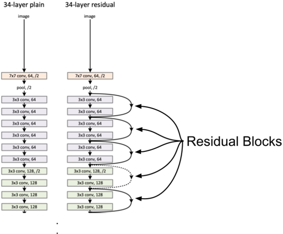
与 AlexNet 相比,ResNet 是一个复杂得多的架构。ResNet 代表残差神经网络(Residual Neural Network),由 K. He、X. Zhang、S. Ren 和 J. Sun 在 2015 年的论文《Deep residual learning for image recognition》中提出。ResNet 由残差块(residual block)组成,残差块通过跳过中间的某些层,将知识从一层传递到更远的层。这种层的连接被称为跳跃连接(skip-connections),因为我们跳过了一层或多层。跳跃连接通过将梯度传播到更远的层来帮助解决梯度消失问题。这使我们能够训练非常大的卷积神经网络而不会损失性能。通常,如果我们使用大型神经网络,训练损失会在某个点上升,但使用跳跃连接可以防止这种情况。图 7 可以更好地说明这一点。
图 7:简单卷积网络与残差卷积网络的对比 10。注意跳跃连接。请注意,此图中省略了最后的层。
10 K. He, X. Zhang, S. Ren and J. Sun, Deep residual learning for image recognition, 2015
残差块很容易理解。你从某一层取出输出,跳过一些层,再将该输出加到网络中更远的某一层上。虚线表示需要调整输入形状,因为使用了最大池化,而最大池化的使用会改变输出的大小。
ResNet 有许多不同的变体:18、34、50、101 和 152 层,所有这些变体都有在 ImageNet 数据集上预训练好的权重。如今,预训练模型几乎适用于(几乎)所有任务,但请确保你从小模型开始,例如,从 resnet-18 开始,而不是 resnet-50。其他一些 ImageNet 预训练模型包括:
- Inception
- DenseNet(不同的变体)
- NASNet
- PNASNet
- VGG
- Xception
- ResNeXt
- EfficientNet,等等。
大多数预训练的最先进模型都可以在 GitHub 上的 pytorchpretrainedmodels 仓库中找到:https://github.com/Cadene/pretrainedmodels.pytorch。详细讨论这些模型超出了本章(以及本书)的范围。由于我们只看应用,让我们看看这样的预训练模型如何用于分割任务。
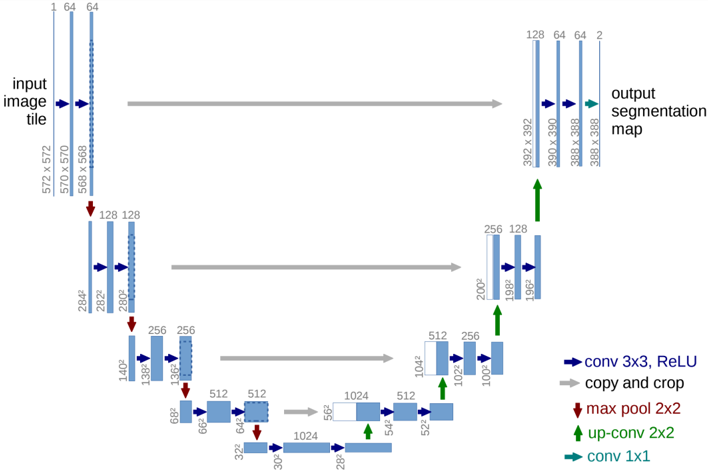
图 8:U-Net 架构 11。
11 O. Ronneberger, P. Fischer and T. Brox. U-Net: Convolutional networks for biomedical image segmentation. In MICCAI, 2015
分割(segmentation)是计算机视觉中非常流行的任务。在分割任务中,我们试图把前景从背景中移除/提取出来。前景和背景可以有不同定义。我们也可以说这是一个逐像素分类(pixel-wise classification)任务,你的工作是为给定图像中的每个像素分配一个类别。我们正在处理的气胸数据集实际上就是一个分割任务。在这个任务中,给定胸部 X 光图像,我们需要分割出气胸区域。分割任务中最流行的模型是 U-Net。其结构如图 8 所示。
U-Net 有两个部分:编码器(encoder)和解码器(decoder)。编码器和你目前见过的任何卷积网络一样。解码器则有点不同。解码器由反卷积(上卷积,up-convolution)层组成。在上卷积(转置卷积,transposed convolution)中,我们使用的滤波器在应用于小图像时会产生更大的图像。在 PyTorch 中,你可以使用 ConvTranspose2d 进行这种操作。必须注意,上卷积与上采样(up-sampling)不是一回事。上采样是一个简单的过程,我们对图像应用一个函数来调整其大小。而在上卷积中,我们学习滤波器。我们把编码器的某些部分作为某些解码器的输入。这对上卷积层很重要。
让我们看看这个 U-Net 是如何实现的。
# simple_unet.py
import torch
import torch.nn as nn
from torch.nn import functional as F


def double_conv(in_channels, out_channels):
    """
    This function applies two convolutional layers each followed by a ReLU activation function

    :param in_channels: number of input channels
    :param out_channels: number of output channels
    :return: a down-conv layer
    """
    conv = nn.Sequential(
        nn.Conv2d(in_channels, out_channels, kernel_size=3),
        nn.ReLU(inplace=True),
        nn.Conv2d(out_channels, out_channels, kernel_size=3),
        nn.ReLU(inplace=True),
    )
    return conv


def crop_tensor(tensor, target_tensor):
    """
    Center crops a tensor to size of a given target tensor size

    Please note that this function is applicable only to this implementation of unet.
    There are a few assumptions in this implementation that might not be applicable
    to all networks and all other use-cases.

    Both tensors are of shape (bs, c, h, w)

    :param tensor: a tensor that needs to be cropped
    :param target_tensor: target tensor of smaller size
    :return: cropped tensor
    """
    target_size = target_tensor.size()[2]
    tensor_size = tensor.size()[2]
    delta = tensor_size - target_size
    delta = delta // 2
    return tensor[
        :, :, delta : tensor_size - delta, delta : tensor_size - delta
    ]


class UNet(nn.Module):
    def __init__(self):
        super(UNet, self).__init__()
        # we need only one max_pool as it is not learned
        self.max_pool_2x2 = nn.MaxPool2d(kernel_size=2, stride=2)

        self.down_conv_1 = double_conv(1, 64)
        self.down_conv_2 = double_conv(64, 128)
        self.down_conv_3 = double_conv(128, 256)
        self.down_conv_4 = double_conv(256, 512)
        self.down_conv_5 = double_conv(512, 1024)

        self.up_trans_1 = nn.ConvTranspose2d(
            in_channels=1024,
            out_channels=512,
            kernel_size=2,
            stride=2,
        )
        self.up_conv_1 = double_conv(1024, 512)

        self.up_trans_2 = nn.ConvTranspose2d(
            in_channels=512,
            out_channels=256,
            kernel_size=2,
            stride=2,
        )
        self.up_conv_2 = double_conv(512, 256)

        self.up_trans_3 = nn.ConvTranspose2d(
            in_channels=256,
            out_channels=128,
            kernel_size=2,
            stride=2,
        )
        self.up_conv_3 = double_conv(256, 128)

        self.up_trans_4 = nn.ConvTranspose2d(
            in_channels=128,
            out_channels=64,
            kernel_size=2,
            stride=2,
        )
        self.up_conv_4 = double_conv(128, 64)

        self.out = nn.Conv2d(
            in_channels=64,
            out_channels=2,
            kernel_size=1,
        )

    def forward(self, image):
        # encoder
        x1 = self.down_conv_1(image)
        x2 = self.max_pool_2x2(x1)
        x3 = self.down_conv_2(x2)
        x4 = self.max_pool_2x2(x3)
        x5 = self.down_conv_3(x4)
        x6 = self.max_pool_2x2(x5)
        x7 = self.down_conv_4(x6)
        x8 = self.max_pool_2x2(x7)
        x9 = self.down_conv_5(x8)

        # decoder
        x = self.up_trans_1(x9)
        y = crop_tensor(x7, x)
        x = self.up_conv_1(torch.cat([x, y], axis=1))

        x = self.up_trans_2(x)
        y = crop_tensor(x5, x)
        x = self.up_conv_2(torch.cat([x, y], axis=1))

        x = self.up_trans_3(x)
        y = crop_tensor(x3, x)
        x = self.up_conv_3(torch.cat([x, y], axis=1))

        x = self.up_trans_4(x)
        y = crop_tensor(x1, x)
        x = self.up_conv_4(torch.cat([x, y], axis=1))

        # output layer
        out = self.out(x)
        return out


if __name__ == "__main__":
    image = torch.rand((1, 1, 572, 572))
    model = UNet()
    print(model(image))
请注意,我上面展示的 U-Net 实现是 U-Net 论文的原始实现。网上可以找到许多变体。有些人喜欢用双线性采样代替转置卷积进行上采样,但那不是论文的真正实现。不过它可能表现更好。在上面显示的原始实现中,输入是单通道图像,输出有两个通道:一个用于前景,一个用于背景。如你所见,这可以很容易地定制为任意数量的类别和任意数量的输入通道。在这个实现中,输入图像大小与输出图像大小不同,因为我们使用的卷积没有填充。
我们看到 U-Net 的编码器部分不过是一个简单的卷积网络。因此,我们可以用任何网络(如 ResNet)替换它。替换时也可以使用预训练权重。这样,我们就可以使用一个在 ImageNet 上预训练的基于 ResNet 的编码器和一个通用的解码器。除了 ResNet,还可以使用许多不同的网络架构。Pavel Yakubovskiy 的 Segmentation Models Pytorch 12 就是许多这类变体的实现,其中编码器可以被预训练模型替换。让我们将基于 ResNet 的 U-Net 应用于气胸检测问题。
12 https://github.com/qubvel/segmentation_models.pytorch
大多数此类问题应该有两个输入:原始图像和掩码(mask)。在多个物体的情况下,会有多个掩码。在我们的气胸数据集中,提供的是 RLE 而不是掩码。RLE 代表运行长度编码(run-length encoding),是一种表示二值掩码以节省空间的方式。深入讲解 RLE 超出了本章的范围。所以,让我们假设我们有一张输入图像和对应的掩码。让我们先设计一个输出图像和掩码图像的数据集类。请注意,我们将以这样的方式创建这些脚本,使它们几乎可以应用于任何分割问题。训练数据集是一个 CSV 文件,只包含图像 ID,这些 ID 也是文件名。
# dataset.py
import os
import glob
import torch
import numpy as np
import pandas as pd
from PIL import Image, ImageFile
from tqdm import tqdm
from collections import defaultdict
from torchvision import transforms
from albumentations import (
    Compose,
    OneOf,
    RandomBrightnessContrast,
    RandomGamma,
    ShiftScaleRotate,
)

ImageFile.LOAD_TRUNCATED_IMAGES = True


class SIIMDataset(torch.utils.data.Dataset):
    def __init__(
        self,
        image_ids,
        transform=True,
        preprocessing_fn=None,
    ):
        """
        Dataset class for segmentation problem

        :param image_ids: ids of the images, list
        :param transform: True/False, no transform in validation
        :param preprocessing_fn: a function for preprocessing image
        """
        # we create a empty dictionary to store iamge
        # and mask paths
        self.data = defaultdict(dict)
        # for augmentations
        self.transform = transform
        # preprocessing function to normalize
        # images
        self.preprocessing_fn = preprocessing_fn
        # albumentation augmentations
        # we have shift, scale & rotate
        # applied with 80% probability
        # and then one of gamma and brightness/contrast
        # is applied to the image
        # albumentation takes care of which augmentation
        # is applied to image and mask
        self.aug = Compose(
            [
                ShiftScaleRotate(
                    shift_limit=0.0625,
                    scale_limit=0.1,
                    rotate_limit=10,
                    p=0.8,
                ),
                OneOf(
                    [
                        RandomGamma(
                            gamma_limit=(90, 110)
                        ),
                        RandomBrightnessContrast(
                            brightness_limit=0.1,
                            contrast_limit=0.1,
                        ),
                    ],
                    p=0.5,
                ),
            ]
        )

        # going over all image_ids to store
        # image and mask paths
        for imgid in image_ids:
            files = glob.glob(os.path.join(TRAIN_PATH, imgid, "*.png"))
            self.data[counter] = {
                "img_path": os.path.join(
                    TRAIN_PATH, imgid + ".png"
                ),
                "mask_path": os.path.join(
                    TRAIN_PATH, imgid + "_mask.png"
                ),
            }

    def __len__(self):
        # return length of dataset
        return len(self.data)

    def __getitem__(self, item):
        # for a given item index,
        # return image and mask tensors

        # read image and mask paths
        img_path = self.data[item]["img_path"]
        mask_path = self.data[item]["mask_path"]

        # read image and convert to RGB
        img = Image.open(img_path)
        img = img.convert("RGB")

        # PIL image to numpy array
        img = np.array(img)

        # read mask image
        mask = Image.open(mask_path)
        # convert to binary float matrix
        mask = (mask >= 1).astype("float32")

        # if this is training data, apply transforms
        if self.transform is True:
            augmented = self.aug(image=img, mask=mask)
            img = augmented["image"]
            mask = augmented["mask"]

        # preprocess the image using provided
        # preprocessing tensors. this is basically
        # image normalization
        img = self.preprocessing_fn(img)

        # return image and mask tensors
        return {
            "image": transforms.ToTensor()(img),
            "mask": transforms.ToTensor()(mask).float(),
        }
有了数据集类之后,我们就可以创建训练函数了。
# train.py
import os
import sys
import torch
import numpy as np
import pandas as pd
import segmentation_models_pytorch as smp
import torch.nn as nn
import torch.optim as optim
from apex import amp
from collections import OrderedDict
from sklearn import model_selection
from tqdm import tqdm
from torch.optim import lr_scheduler
from dataset import SIIMDataset

# training csv file path
TRAINING_CSV = "../input/train_pneumothorax.csv"

# training and test batch sizes
TRAINING_BATCH_SIZE = 16
TEST_BATCH_SIZE = 4

# number of epochs
EPOCHS = 10

# define the encoder for U-Net
# check: https://github.com/qubvel/segmentation_models.pytorch
# for all supported encoders
ENCODER = "resnet18"

# we use imagenet pretrained weights for the encoder
ENCODER_WEIGHTS = "imagenet"

# train on gpu
DEVICE = "cuda"


def train(dataset, data_loader, model, criterion, optimizer):
    """
    training function that trains for one epoch

    :param dataset: dataset class (SIIMDataset)
    :param data_loader: torch dataset loader
    :param model: model
    :param criterion: loss function
    :param optimizer: adam, sgd, etc.
    """
    # put the model in train mode
    model.train()

    # calculate number of batches
    num_batches = int(len(dataset) / data_loader.batch_size)

    # init tqdm to track progress
    tk0 = tqdm(data_loader, total=num_batches)

    # loop over all batches
    for d in tk0:
        # fetch input images and masks
        # from dataset batch
        inputs = d["image"]
        targets = d["mask"]

        # move images and masks to cpu/gpu device
        inputs = inputs.to(DEVICE, dtype=torch.float)
        targets = targets.to(DEVICE, dtype=torch.float)

        # zero grad the optimizer
        optimizer.zero_grad()

        # forward step of model
        outputs = model(inputs)

        # calculate loss
        loss = criterion(outputs, targets)

        # backward loss is calculated on a scaled loss
        # context since we are using mixed precision training
        # if you are not using mixed precision training,
        # you can use loss.backward() and delete the following
        # two lines of code
        with amp.scale_loss(loss, optimizer) as scaled_loss:
            scaled_loss.backward()

        # step the optimizer
        optimizer.step()

    # close tqdm
    tk0.close()


def evaluate(dataset, data_loader, model):
    """
    evaluation function to calculate loss on validation set for one epoch

    :param dataset: dataset class (SIIMDataset)
    :param data_loader: torch dataset loader
    :param model: model
    """
    # put model in eval mode
    model.eval()

    # init final_loss to 0
    final_loss = 0

    # calculate number of batches and init tqdm
    num_batches = int(len(dataset) / data_loader.batch_size)
    tk0 = tqdm(data_loader, total=num_batches)

    # we need no_grad context of torch. this save memory
    with torch.no_grad():
        for d in tk0:
            inputs = d["image"]
            targets = d["mask"]

            inputs = inputs.to(DEVICE, dtype=torch.float)
            targets = targets.to(DEVICE, dtype=torch.float)

            output = model(inputs)
            loss = criterion(output, targets)

            # add loss to final loss
            final_loss += loss

    # close tqdm
    tk0.close()

    # return average loss over all batches
    return final_loss / num_batches


if __name__ == "__main__":
    # read the training csv file
    df = pd.read_csv(TRAINING_CSV)

    # split data into training and validation
    df_train, df_valid = model_selection.train_test_split(
        df, random_state=42, test_size=0.1
    )

    # training and validation images lists/arrays
    training_images = df_train.image_id.values
    validation_images = df_valid.image_id.values

    # fetch unet model from segmentation models
    # with specified encoder architecture
    model = smp.Unet(
        encoder_name=ENCODER,
        encoder_weights=ENCODER_WEIGHTS,
        classes=1,
        activation=None,
    )

    # segmentation model provides you with a preprocessing
    # function that can be used for normalizing images
    # normalization is only applied on images and not masks
    prep_fn = smp.encoders.get_preprocessing_fn(
        ENCODER, ENCODER_WEIGHTS
    )

    # send model to device
    model.to(DEVICE)

    # init training dataset
    # transform is True for training data
    train_dataset = SIIMDataset(
        training_images,
        transform=True,
        preprocessing_fn=prep_fn,
    )

    # wrap training dataset in torch's dataloader
    train_loader = torch.utils.data.DataLoader(
        train_dataset,
        batch_size=TRAINING_BATCH_SIZE,
        shuffle=True,
        num_workers=12,
    )

    # init validation dataset
    # augmentations is disabled
    valid_dataset = SIIMDataset(
        validation_images,
        transform=False,
        preprocessing_fn=prep_fn,
    )

    # wrap validation dataset in torch's dataloader
    valid_loader = torch.utils.data.DataLoader(
        valid_dataset,
        batch_size=TEST_BATCH_SIZE,
        shuffle=True,
        num_workers=4
    )

    # NOTE: define the criterion here
    # this is left as an excercise
    # code won't work without defining this
    # criterion = ……

    # we will use Adam optimizer for faster convergence
    optimizer = torch.optim.Adam(model.parameters(), lr=1e-3)

    # reduce learning rate when we reach a plateau on loss
    scheduler = lr_scheduler.ReduceLROnPlateau(
        optimizer, mode="min", patience=3, verbose=True
    )

    # wrap model and optimizer with NVIDIA's apex
    # this is used for mixed precision training
    # if you have a GPU that supports mixed precision,
    # this is very helpful as it will allow us to fit larger images
    # and larger batches
    model, optimizer = amp.initialize(
        model, optimizer, opt_level="O1", verbosity=0
    )

    # if we have more than one GPU, we can use both of them!
    if torch.cuda.device_count() > 1:
        print(f"Let's use {torch.cuda.device_count()} GPUs!")
        model = nn.DataParallel(model)

    # some logging
    print(f"Training batch size: {TRAINING_BATCH_SIZE}")
    print(f"Test batch size: {TEST_BATCH_SIZE}")
    print(f"Epochs: {EPOCHS}")
    print(f"Image size: {IMAGE_SIZE}")
    print(f"Number of training images: {len(train_dataset)}")
    print(f"Number of validation images: {len(valid_dataset)}")
    print(f"Encoder: {ENCODER}")

    # loop over all epochs
    for epoch in range(EPOCHS):
        print(f"Training Epoch: {epoch}")
        # train for one epoch
        train(
            train_dataset,
            train_loader,
            model,
            criterion,
            optimizer,
        )
        print(f"Validation Epoch: {epoch}")
        # calculate validation loss
        val_log = evaluate(
            valid_dataset,
            valid_loader,
            model,
        )
        # step the scheduler
        scheduler.step(val_log["loss"])
        print("\n")
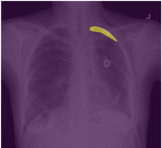
在分割问题中,你可以使用各种损失函数,例如逐像素二值交叉熵、焦点损失(focal loss)、Dice 损失(dice loss)等。我把选择合适的损失函数留给读者根据评估指标来决定。当你训练这样的模型时,你会得到一个试图预测气胸位置的模型,如图 9 所示。在上面的代码中,我们使用了 NVIDIA apex 进行混合精度训练(mixed precision training)。请注意,从 PyTorch 1.6.0+ 版本开始,这已原生可用。
图 9:训练模型检测气胸的示例(可能不是正确的预测)。
我把一些常用的函数放到了一个名为 Well That’s Fantastic Machine Learning (WTFML) 的 Python 包中。让我们看看它如何帮助我们为 FGVC 2020 植物病理学挑战赛 13 的植物图像构建一个多类分类模型。
13 Ranjita Thapa, Noah Snavely, Serge Belongie, Awais Khan. The Plant Pathology 2020 challenge dataset to classify foliar disease of apples. ArXiv e-prints
import os
import pandas as pd
import numpy as np
import albumentations
import argparse
import torch
import torchvision
import torch.nn as nn
import torch.nn.functional as F
from sklearn import metrics
from sklearn.model_selection import train_test_split
from wtfml.engine import Engine
from wtfml.data_loaders.image import ClassificationDataLoader


class DenseCrossEntropy(nn.Module):
    # Taken from:
    # https://www.kaggle.com/pestipeti/plant-pathology-2020-pytorch
    def __init__(self):
        super(DenseCrossEntropy, self).__init__()

    def forward(self, logits, labels):
        logits = logits.float()
        labels = labels.float()
        logprobs = F.log_softmax(logits, dim=-1)
        loss = -labels * logprobs
        loss = loss.sum(-1)
        return loss.mean()


class Model(nn.Module):
    def __init__(self):
        super().__init__()
        self.base_model = torchvision.models.resnet18(pretrained=True)
        in_features = self.base_model.fc.in_features
        self.out = nn.Linear(in_features, 4)

    def forward(self, image, targets=None):
        batch_size, C, H, W = image.shape
        x = self.base_model.conv1(image)
        x = self.base_model.bn1(x)
        x = self.base_model.relu(x)
        x = self.base_model.maxpool(x)
        x = self.base_model.layer1(x)
        x = self.base_model.layer2(x)
        x = self.base_model.layer3(x)
        x = self.base_model.layer4(x)
        x = F.adaptive_avg_pool2d(x, 1).reshape(batch_size, -1)
        x = self.out(x)

        loss = None
        if targets is not None:
            loss = DenseCrossEntropy()(x, targets.type_as(x))
        return x, loss


if __name__ == "__main__":
    parser = argparse.ArgumentParser()
    parser.add_argument(
        "--data_path",
        type=str,
    )
    parser.add_argument(
        "--device",
        type=str,
    )
    parser.add_argument(
        "--epochs",
        type=int,
    )
    args = parser.parse_args()

    df = pd.read_csv(os.path.join(args.data_path, "train.csv"))
    images = df.image_id.values.tolist()
    images = [
        os.path.join(args.data_path, "images", i + ".jpg")
        for i in images
    ]
    targets = df[["healthy", "multiple_diseases", "rust", "scab"]].values

    model = Model()
    model.to(args.device)

    mean = (0.485, 0.456, 0.406)
    std = (0.229, 0.224, 0.225)

    aug = albumentations.Compose(
        [
            albumentations.Normalize(
                mean,
                std,
                max_pixel_value=255.0,
                always_apply=True,
            )
        ]
    )

    (
        train_images,
        valid_images,
        train_targets,
        valid_targets,
    ) = train_test_split(images, targets)

    train_loader = ClassificationDataLoader(
        image_paths=train_images,
        targets=train_targets,
        resize=(128, 128),
        augmentations=aug,
    ).fetch(
        batch_size=16,
        num_workers=4,
        drop_last=False,
        shuffle=True,
        tpu=False,
    )

    valid_loader = ClassificationDataLoader(
        image_paths=valid_images,
        targets=valid_targets,
        resize=(128, 128),
        augmentations=aug,
    ).fetch(
        batch_size=16,
        num_workers=4,
        drop_last=False,
        shuffle=False,
        tpu=False,
    )

    optimizer = torch.optim.Adam(model.parameters(), lr=5e-4)
    scheduler = torch.optim.lr_scheduler.StepLR(
        optimizer, step_size=15, gamma=0.6
    )

    for epoch in range(args.epochs):
        train_loss = Engine.train(
            train_loader, model, optimizer, device=args.device
        )
        valid_loss = Engine.evaluate(
            valid_loader, model, device=args.device
        )
        print(
            f"{epoch}, Train Loss={train_loss} Valid Loss={valid_loss}"
        )
有了数据 14 之后,你可以这样运行脚本:
❯ python plant.py --data_path ../../plant_pathology --device cuda -epochs 2
100%|█████████████| 86/86 [00:12<00:00, 6.73it/s, loss=0.723]
100%|█████████████ 29/29 [00:04<00:00, 6.62it/s, loss=0.433]
0, Train Loss=0.7228777609592261 Valid Loss=0.4327834551704341
100%|█████████████| 86/86 [00:12<00:00, 6.74it/s, loss=0.271]
100%|█████████████ 29/29 [00:04<00:00, 6.63it/s, loss=0.568]
1, Train Loss=0.2708700496790021 Valid Loss=0.56841839541649
如你所见,这如何让我们的生活更简单,让代码更易读、易理解。不带任何包装的 PyTorch 效果最好。图像领域远不止分类,如果我把它们都写出来,我就得再写一本书了。所以,我决定这样做:写一本《Approaching (Almost) Any Image Problem》(接近(几乎)任何图像问题)。