超参数优化
强大的模型随之而来的是优化超参数(hyperparameters)以获得最佳得分模型的巨大问题。那么,什么是超参数优化(hyperparameter optimization)呢?假设你的机器学习项目有一个简单的流水线(pipeline)。有一个数据集,你直接应用一个模型,然后你就有了结果。模型在这里所拥有的参数被称为超参数,即控制模型训练/拟合过程的参数。如果我们用 SGD 训练线性回归,模型的参数是斜率和截距,超参数是学习率。你会注意到,我在本章以及整本书中会交替使用这些术语。假设模型中有三个参数 a、b、c,所有这些参数都可以是 1 到 10 之间的整数。这些参数的一个"正确"组合会为你提供最好的结果。所以,这有点像带三位拨号组合锁的手提箱。然而,三位拨号组合锁只有一个正确答案。模型有很多正确答案。那么,你如何找到最佳参数呢?一种方法是评估所有组合,看看哪一种能提升指标。让我们看看这是如何做到的。
# define the best accuracy to be 0
# if you choose loss as a metric,
# you can make best loss to be inf (np.inf)
best_accuracy = 0
best_parameters = {"a": 0, "b": 0, "c": 0}

# loop over all values for a, b & c
for a in range(1, 11):
    for b in range(1, 11):
        for c in range(1, 11):
            # inititalize model with current parameters
            model = MODEL(a, b, c)
            # fit the model
            model.fit(training_data)
            # make predictions
            preds = model.predict(validation_data)
            # calculate accuracy
            accuracy = metrics.accuracy_score(targets, preds)
            # save params if current accuracy
            # is greater than best accuracy
            if accuracy > best_accuracy:
                best_accuracy = accuracy
                best_parameters["a"] = a
                best_parameters["b"] = b
                best_parameters["c"] = c
在上面的代码中,我们遍历了从 1 到 10 的所有参数。所以,我们总共有 1000(\(10 \times 10 \times 10\))次模型拟合。嗯,这可能会很昂贵,因为模型训练可能需要很长时间。在这种情形下,这或许还可以接受,但在现实世界的场景中,不仅参数不止三个,而且每个参数的值也不止十个。大多数模型的参数是实数值,不同参数的组合可以是无限的。
让我们看看 scikit-learn 中的随机森林(random forest)模型。
RandomForestClassifier(
n_estimators=100,
criterion='gini',
max_depth=None,
min_samples_split=2,
min_samples_leaf=1,
min_weight_fraction_leaf=0.0,
max_features='auto',
max_leaf_nodes=None,
min_impurity_decrease=0.0,
min_impurity_split=None,
bootstrap=True,
oob_score=False,
n_jobs=None,
random_state=None,
verbose=0,
warm_start=False,
class_weight=None,
ccp_alpha=0.0,
max_samples=None,
)
这里有十九个参数,所有这些参数在它们可以取的所有值下的所有组合将是无限的。通常,我们没有资源和时间去这样做。因此,我们指定一个参数网格(grid)。在这个网格上搜索以找到最佳参数组合的方法被称为网格搜索(grid search)。我们可以说 n_estimators 可以是 100、200、250、300、400、500;max_depth 可以是 1、2、5、7、11、15;criterion 可以是 gini 或 entropy。这些参数看起来可能不多,但如果数据集太大,计算会花费大量时间。我们可以像之前一样通过创建三个 for 循环并在验证集上计算得分来让网格搜索工作。还必须注意,如果你使用 k 折交叉验证(kfold cross-validation),你需要更多的循环,这意味着需要更多时间来找到完美的参数。因此,网格搜索并不十分流行。让我们通过一个根据手机规格预测手机价格区间的例子来看看它是如何完成的。
图 1:手机价格数据集快照
| 电池电量 | 蓝牙 | 时钟速度 | 双卡 | 前置摄像头 | 4G | 内存 | 厚度 | 价格区间 |
|---|---|---|---|---|---|---|---|---|
| 842 | 0 | 2.2 | 0 | 1 | 0 | 7 | 0.6 | 1 |
| 1021 | 1 | 0.5 | 1 | 0 | 1 | 53 | 0.7 | 2 |
| 563 | 1 | 0.5 | 1 | 2 | 1 | 41 | 0.9 | 2 |
| 615 | 1 | 2.5 | 0 | 0 | 0 | 10 | 0.8 | 2 |
| 1821 | 1 | 1.2 | 0 | 13 | 1 | 44 | 0.6 | 1 |
| 794 | 1 | 0.5 | 1 | 0 | 1 | 2 | 0.8 | 0 |
| 1965 | 1 | 2.6 | 1 | 0 | 0 | 39 | 0.2 | 2 |
7 https://www.kaggle.com/iabhishekofficial/mobile-price-classification
我们有 20 个特征,如双卡(dual sim)、电池电量(battery power)等,以及一个价格区间,它有从 0 到 3 的 4 个类别。训练集中只有 2000 个样本。我们可以轻松地使用分层 k 折交叉验证(stratified kfold)并以准确率(accuracy)作为评估指标。我们将使用具有上述参数范围的随机森林模型,看看如何在下面的例子中进行网格搜索。
# rf_grid_search.py
import numpy as np
import pandas as pd
from sklearn import ensemble
from sklearn import metrics
from sklearn import model_selection

if __name__ == "__main__":
    # read the training data
    df = pd.read_csv("../input/mobile_train.csv")

    # features are all columns without price_range
    # note that there is no id column in this dataset
    # here we have training features
    X = df.drop("price_range", axis=1).values

    # and the targets
    y = df.price_range.values

    # define the model here
    # i am using random forest with n_jobs=-1
    # n_jobs=-1 => use all cores
    classifier = ensemble.RandomForestClassifier(n_jobs=-1)

    # define a grid of parameters
    # this can be a dictionary or a list of
    # dictionaries
    param_grid = {
        "n_estimators": [100, 200, 250, 300, 400, 500],
        "max_depth": [1, 2, 5, 7, 11, 15],
        "criterion": ["gini", "entropy"]
    }

    # initialize grid search
    # estimator is the model that we have defined
    # param_grid is the grid of parameters
    # we use accuracy as our metric. you can define your own
    # higher value of verbose implies a lot of details are printed
    # cv=5 means that we are using 5 fold cv (not stratified)
    model = model_selection.GridSearchCV(
        estimator=classifier,
        param_grid=param_grid,
        scoring="accuracy",
        verbose=10,
        n_jobs=1,
        cv=5
    )

    # fit the model and extract best score
    model.fit(X, y)
    print(f"Best score: {model.best_score_}")
    print("Best parameters set:")
    best_parameters = model.best_estimator_.get_params()
    for param_name in sorted(param_grid.keys()):
        print(f"\t{param_name}: {best_parameters[param_name]}")
这会打印很多东西,让我们看看最后几行。
[CV]  criterion=entropy, max_depth=15, n_estimators=500, score=0.895, total=   1.0s
[CV] criterion=entropy, max_depth=15, n_estimators=500 ...............
[CV]  criterion=entropy, max_depth=15, n_estimators=500, score=0.890, total=   1.1s
[CV] criterion=entropy, max_depth=15, n_estimators=500 ...............
[CV]  criterion=entropy, max_depth=15, n_estimators=500, score=0.910, total=   1.1s
[CV] criterion=entropy, max_depth=15, n_estimators=500 ...............
[CV]  criterion=entropy, max_depth=15, n_estimators=500, score=0.880, total=   1.1s
[CV] criterion=entropy, max_depth=15, n_estimators=500 ...............
[CV]  criterion=entropy, max_depth=15, n_estimators=500, score=0.870, total=   1.1s
[Parallel(n_jobs=1)]: Done 360 out of 360 | elapsed:  3.7min finished
Best score: 0.889
Best parameters set:
criterion: 'entropy'
max_depth: 15
n_estimators: 500
最后,我们看到我们最好的五折准确率得分是 0.889,并且我们从网格搜索中得到了最佳参数。接下来我们可以使用的下一个好方法就是随机搜索(random search)。在随机搜索中,我们随机选择一组参数组合并计算交叉验证得分。这里消耗的时间比网格搜索少,因为我们不会评估所有不同的参数组合。我们选择要评估模型的次数,而这决定了搜索需要多少时间。代码与上面的没有太大不同。除了 GridSearchCV 之外,我们使用 RandomizedSearchCV。
# rf_random_search.py
import numpy as np
import pandas as pd
from sklearn import ensemble
from sklearn import metrics
from sklearn import model_selection

if __name__ == "__main__":
    . . .
    # define the model here
    # i am using random forest with n_jobs=-1
    # n_jobs=-1 => use all cores
    classifier = ensemble.RandomForestClassifier(n_jobs=-1)

    # define a grid of parameters
    # this can be a dictionary or a list of
    # dictionaries
    param_grid = {
        "n_estimators": np.arange(100, 1500, 100),
        "max_depth": np.arange(1, 31),
        "criterion": ["gini", "entropy"]
    }

    # initialize random search
    # estimator is the model that we have defined
    # param_distributions is the grid/distribution of parameters
    # we use accuracy as our metric. you can define your own
    # higher value of verbose implies a lot of details are printed
    # cv=5 means that we are using 5 fold cv (not stratified)
    # n_iter is the number of iterations we want
    # if param_distributions has all the values as list,
    # random search will be done by sampling without replacement
    # if any of the parameters come from a distribution,
    # random search uses sampling with replacement
    model = model_selection.RandomizedSearchCV(
        estimator=classifier,
        param_distributions=param_grid,
        n_iter=20,
        scoring="accuracy",
        verbose=10,
        n_jobs=1,
        cv=5
    )

    # fit the model and extract best score
    model.fit(X, y)
    print(f"Best score: {model.best_score_}")
    print("Best parameters set:")
    best_parameters = model.best_estimator_.get_params()
    for param_name in sorted(param_grid.keys()):
        print(f"\t{param_name}: {best_parameters[param_name]}")
我们为随机搜索改变了参数网格,看起来我们甚至稍微改善了结果。
Best score: 0.8905
Best parameters set:
criterion: entropy
max_depth: 25
n_estimators: 300
如果迭代次数更少,随机搜索比网格搜索更快。使用这两种方法,只要模型有 fit 和 predict 函数(这是 scikit-learn 的标准),你就可以为所有类型的模型找到最佳(?)参数。有时,你可能想使用流水线。例如,假设我们正在处理一个多分类(multiclass classification)问题。在这个问题中,训练数据由两个文本列组成,你需要构建一个模型来预测类别。假设你选择的流水线是首先以半监督方式应用 tf-idf,然后使用带 SVM 分类器的 SVD。现在,问题是我们必须选择 SVD 的成分(components),还需要调整 SVM 的参数。如何做到这一点如下面的代码片段所示。
# pipeline_search.py
import numpy as np
import pandas as pd
from sklearn import metrics
from sklearn import model_selection
from sklearn import pipeline
from sklearn.decomposition import TruncatedSVD
from sklearn.feature_extraction.text import TfidfVectorizer
from sklearn.preprocessing import StandardScaler
from sklearn.svm import SVC

def quadratic_weighted_kappa(y_true, y_pred):
    """ Create a wrapper for cohen's kappa with quadratic weights """
    return metrics.cohen_kappa_score(
        y_true,
        y_pred,
        weights="quadratic"
    )

if __name__ == '__main__':
    # Load the training file
    train = pd.read_csv('../input/train.csv')

    # we dont need ID columns
    idx = test.id.values.astype(int)
    train = train.drop('id', axis=1)
    test = test.drop('id', axis=1)

    # create labels. drop useless columns
    y = train.relevance.values

    # do some lambda magic on text columns
    traindata = list(
        train.apply(lambda x:'%s %s' % (x['text1'], x['text2']),axis=1)
    )
    testdata = list(
        test.apply(lambda x:'%s %s' % (x['text1'], x['text2']),axis=1)
    )

    # tfidf vectorizer
    tfv = TfidfVectorizer(
        min_df=3,
        max_features=None,
        strip_accents='unicode',
        analyzer='word',
        token_pattern=r'\w{1,}',
        ngram_range=(1, 3),
        use_idf=1,
        smooth_idf=1,
        sublinear_tf=1,
        stop_words='english'
    )

    # Fit TFIDF
    tfv.fit(traindata)
    X =  tfv.transform(traindata)
    X_test = tfv.transform(testdata)

    # Initialize SVD
    svd = TruncatedSVD()

    # Initialize the standard scaler
    scl = StandardScaler()

    # We will use SVM here..
    svm_model = SVC()

    # Create the pipeline
    clf = pipeline.Pipeline(
        [
            ('svd', svd),
            ('scl', scl),
            ('svm', svm_model)
        ]
    )

    # Create a parameter grid to search for
    # best parameters for everything in the pipeline
    param_grid = {
        'svd__n_components' : [200, 300],
        'svm__C': [10, 12]
    }

    # Kappa Scorer
    kappa_scorer = metrics.make_scorer(
        quadratic_weighted_kappa,
        greater_is_better=True
    )

    # Initialize Grid Search Model
    model = model_selection.GridSearchCV(
        estimator=clf,
        param_grid=param_grid,
        scoring=kappa_scorer,
        verbose=10,
        n_jobs=-1,
        refit=True,
        cv=5
    )

    # Fit Grid Search Model
    model.fit(X, y)
    print("Best score: %0.3f" % model.best_score_)
    print("Best parameters set:")
    best_parameters = model.best_estimator_.get_params()
    for param_name in sorted(param_grid.keys()):
        print("\t%s: %r" % (param_name, best_parameters[param_name]))

    # Get best model
    best_model = model.best_estimator_

    # Fit model with best parameters optimized for QWK
    best_model.fit(X, y)
    preds = best_model.predict(...)
这里展示的流水线有 SVD(奇异值分解,Singular Value Decomposition)、标准缩放(standard scaling)和一个 SVM(支持向量机,Support Vector Machines)模型。请注意,由于训练数据不可用,你无法按原样运行上述代码。
当我们进入更高级的超参数优化技术时,我们可以看看使用不同类型的极小化(minimization)算法来极小化函数。这可以通过使用许多极小化函数来实现,例如下山单纯形算法(downhill simplex algorithm)、Nelder-Mead 优化、使用带高斯过程(Gaussian process)的贝叶斯技术来寻找最佳参数,或者使用遗传算法(genetic algorithm)。我将在集成(ensembling)和堆叠(stacking)章节中更多地讨论下山单纯形和 Nelder-Mead 的应用。首先,让我们看看高斯过程如何用于超参数优化。这类算法需要一个它们可以优化的函数。大多数时候,这是关于这个函数的极小化,就像我们极小化损失(loss)一样。
所以,假设你想为最佳准确率找到最佳参数,显然准确率越高越好。现在我们无法极小化准确率,但当我们将它乘以 -1 时,我们就可以极小化它。这样,我们是在极小化准确率的相反数,但实际上,我们是在最大化准确率。使用带高斯过程的贝叶斯优化(Bayesian optimization)可以通过使用 scikit-optimize(skopt)库中的 gp_minimize 函数来完成。让我们看看如何使用这个函数来调整我们的随机森林模型的参数。
# rf_gp_minimize.py
import numpy as np
import pandas as pd
from functools import partial
from sklearn import ensemble
from sklearn import metrics
from sklearn import model_selection
from skopt import gp_minimize
from skopt import space

def optimize(params, param_names, x, y):
    """ The main optimization function. This function takes all the arguments from the search space and training features and targets. It then initializes
    the models by setting the chosen parameters and runs cross-validation and returns a negative accuracy score
    :param params: list of params from gp_minimize
    :param param_names: list of param names. order is important!
    :param x: training data
    :param y: labels/targets
    :return: negative accuracy after 5 folds
    """
    # convert params to dictionary
    params = dict(zip(param_names, params))

    # initialize model with current parameters
    model = ensemble.RandomForestClassifier(**params)

    # initialize stratified k-fold
    kf = model_selection.StratifiedKFold(n_splits=5)

    # initialize accuracy list
    accuracies = []

    # loop over all folds
    for idx in kf.split(X=x, y=y):
        train_idx, test_idx = idx[0], idx[1]
        xtrain = x[train_idx]
        ytrain = y[train_idx]
        xtest = x[test_idx]
        ytest = y[test_idx]

        # fit model for current fold
        model.fit(xtrain, ytrain)

        #create predictions
        preds = model.predict(xtest)

        # calculate and append accuracy
        fold_accuracy = metrics.accuracy_score(
            ytest,
            preds
        )
        accuracies.append(fold_accuracy)

    # return negative accuracy
    return -1 * np.mean(accuracies)

if __name__ == "__main__":
    # read the training data
    df = pd.read_csv("../input/mobile_train.csv")

    # features are all columns without price_range
    # note that there is no id column in this dataset
    # here we have training features
    X = df.drop("price_range", axis=1).values

    # and the targets
    y = df.price_range.values

    # define a parameter space
    param_space = [
        # max_depth is an integer between 3 and 10
        space.Integer(3, 15, name="max_depth"),
        # n_estimators is an integer between 50 and 1500
        space.Integer(100, 1500, name="n_estimators"),
        # criterion is a category. here we define list of categories
        space.Categorical(["gini", "entropy"], name="criterion"),
        # you can also have Real numbered space and define a
        # distribution you want to pick it from
        space.Real(0.01, 1, prior="uniform", name="max_features")
    ]

    # make a list of param names
    # this has to be same order as the search space
    # inside the main function
    param_names = [
        "max_depth",
        "n_estimators",
        "criterion",
        "max_features"
    ]

    # by using functools partial, i am creating a
    # new function which has same parameters as the
    # optimize function except for the fact that
    # only one param, i.e. the "params" parameter is
    # required. this is how gp_minimize expects the
    # optimization function to be. you can get rid of this
    # by reading data inside the optimize function or by
    # defining the optimize function here.
    optimization_function = partial(
        optimize,
        param_names=param_names,
        x=X,
        y=y
    )

    # now we call gp_minimize from scikit-optimize
    # gp_minimize uses bayesian optimization for
    # minimization of the optimization function.
    # we need a space of parameters, the function itself,
    # the number of calls/iterations we want to have
    result = gp_minimize(
        optimization_function,
        dimensions=param_space,
        n_calls=15,
        n_random_starts=10,
        verbose=10
    )

    # create best params dict and print it
    best_params = dict(
        zip(
            param_names,
            result.x
        )
    )
    print(best_params)
同样,这会生成大量输出,其最后部分如下所示。
Iteration No: 14 started. Searching for the next optimal point.
Iteration No: 14 ended. Search finished for the next optimal point.
Time taken: 4.7793
Function value obtained: -0.9075
Current minimum: -0.9075
Iteration No: 15 started. Searching for the next optimal point.
Iteration No: 15 ended. Search finished for the next optimal point.
Time taken: 49.4186
Function value obtained: -0.9075
Current minimum: -0.9075
{'max_depth': 12, 'n_estimators': 100, 'criterion': 'entropy', 'max_features': 1.0}
看起来我们已经设法突破了 0.90 的准确率。这真是太棒了!
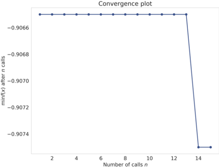
我们还可以通过下面的代码片段来查看(绘制)我们是如何实现收敛的。
from skopt.plots import plot_convergence
plot_convergence(result)
收敛图如图 2 所示。
图 2:随机森林参数优化的收敛图
有很多库提供超参数优化。scikit-optimize 就是你可以使用的这样一个库。另一个有用的超参数优化库是 hyperopt。hyperopt 使用树结构 Parzen 估计器(Tree-structured Parzen Estimator,TPE)来找到最优参数。看看下面的代码片段,我在其中使用 hyperopt 对之前的代码做了最小改动。
# rf_hyperopt.py
import numpy as np
import pandas as pd
from functools import partial
from sklearn import ensemble
from sklearn import metrics
from sklearn import model_selection
from hyperopt import hp, fmin, tpe, Trials
from hyperopt.pyll.base import scope

def optimize(params, x, y):
    """ The main optimization function. This function takes all the arguments from the search space and training features and targets. It then initializes
    the models by setting the chosen parameters and runs cross-validation and returns a negative accuracy score
    :param params: dict of params from hyperopt
    :param x: training data
    :param y: labels/targets
    :return: negative accuracy after 5 folds
    """
    # initialize model with current parameters
    model = ensemble.RandomForestClassifier(**params)

    # initialize stratified k-fold
    kf = model_selection.StratifiedKFold(n_splits=5)
    . . .

    # return negative accuracy
    return -1 * np.mean(accuracies)

if __name__ == "__main__":
    # read the training data
    df = pd.read_csv("../input/mobile_train.csv")

    # features are all columns without price_range
    # note that there is no id column in this dataset
    # here we have training features
    X = df.drop("price_range", axis=1).values

    # and the targets
    y = df.price_range.values

    # define a parameter space
    # now we use hyperopt
    param_space = {
        # quniform gives round(uniform(low, high) / q) * q
        # we want int values for depth and estimators
        "max_depth": scope.int(hp.quniform("max_depth", 1, 15, 1)),
        "n_estimators": scope.int(
            hp.quniform("n_estimators", 100, 1500, 1)
        ),
        # choice chooses from a list of values
        "criterion": hp.choice("criterion", ["gini", "entropy"]),
        # uniform chooses a value between two values
        "max_features": hp.uniform("max_features", 0, 1)
    }

    # partial function
    optimization_function = partial(
        optimize,
        x=X,
        y=y
    )

    # initialize trials to keep logging information
    trials = Trials()

    # run hyperopt
    hopt = fmin(
        fn=optimization_function,
        space=param_space,
        algo=tpe.suggest,
        max_evals=15,
        trials=trials
    )
    print(hopt)
如你所见,这与之前的代码没有太大不同。你必须以不同的格式定义参数空间,并且还需要通过使用 hyperopt 而不是 gp_minimize 来更改实际的优化部分。结果相当不错!
❯ python rf_hyperopt.py
100%|██████████████████| 15/15 [04:38<00:00, 18.57s/trial, best loss: 0.9095000000000001]
{'criterion': 1, 'max_depth': 11.0, 'max_features': 0.821163568049807, 'n_estimators': 806.0}
我们得到了一个比以前稍微好一点的准确率,以及一组我们可以使用的参数。请注意,最终结果中 criterion 是 1。这意味着选择了选项 1,即 entropy。上述描述的超参数调整方法是最常见的,它们几乎适用于所有模型:线性回归、逻辑回归、基于树的模型、梯度提升模型(如 xgboost、lightgbm),甚至神经网络!
尽管这些方法存在,但要想学习,必须从手动调整超参数开始,即手工调整。手工调整将帮助你学习基础知识,例如,在梯度提升中,当你增加深度时,你应该降低学习率。如果你使用自动化工具,就不可能学到这一点。参考下表了解要调整什么。RS* 表示随机搜索应该更好。
| 模型 | 优化项 | 取值范围 |
|---|---|---|
| Linear Regression | - fit_intercept - normalize | - True/False - True/False |
| Ridge | - alpha - fit_intercept - normalize | - 0.01, 0.1, 1.0, 10, 100 - True/False - True/False |
| k-neighbors | - n_neighbors - p | - 2, 4, 8, 16 …. - 2, 3 |
| SVM | - C - gamma - class_weight | - 0.001,0.01..10..100..1000 - ‘auto’, RS* - ‘balanced’ , None |
| Logistic Regression | - Penalty - C | - l1 or l2 - 0.001, 0.01…..10…100 |
| Lasso | - Alpha - Normalize | - 0.1, 1.0, 10 - True/False |
| Random Forest | - n_estimators - max_depth - min_samples_split - min_samples_leaf - max features | - 120, 300, 500, 800, 1200 - 5, 8, 15, 25, 30, None - 1, 2, 5, 10, 15, 100 - 1, 2, 5, 10 - log2, sqrt, None |
| XGBoost | - eta - gamma - max_depth - min_child_weight - subsample - colsample_bytree - lambda - alpha | - 0.01,0.015, 0.025, 0.05, 0.1 - 0.05-0.1,0.3,0.5,0.7,0.9,1.0 - 3, 5, 7, 9, 12, 15, 17, 25 - 1, 3, 5, 7 - 0.6, 0.7, 0.8, 0.9, 1.0 - 0.6, 0.7, 0.8, 0.9, 1.0 - 0.01-0.1, 1.0 , RS* - 0, 0.1, 0.5, 1.0 RS* |
一旦你更擅长手工调整参数,你可能甚至不需要任何自动化的超参数调整。当你创建大型模型或引入大量特征时,你也会使它容易过拟合(overfitting)训练数据。为了避免过拟合,你需要在训练数据特征中引入噪声或惩罚代价函数(cost function)。这种惩罚被称为正则化(regularization),它有助于模型的泛化。在线性模型中,最常见的正则化类型是 L1 和 L2。L1 也被称为 Lasso 回归(Lasso regression),L2 被称为 Ridge 回归(Ridge regression)。说到神经网络,我们使用弃置(dropout)、添加数据增强(augmentation)、噪声等来正则化我们的模型。使用超参数优化,你也可以找到要使用的正确惩罚。