特征选择
当你创建完成千上万个特征之后,就该从中挑选一些了。当然,我们本就不应该创建成千上万个无用的特征。特征过多会带来一个众所周知的问题——维数灾难(curse of dimensionality)。如果你有大量特征,就必须有大量训练样本来覆盖所有这些特征。什么才算"大量"并没有明确的定义,这需要你自己通过正确地验证模型、检查训练模型所花的时间来摸索。
特征选择最简单的方式是移除方差(variance)极低的特征。如果特征的方差非常低(即非常接近 0),说明它几乎是个常量,因而对任何模型都没有任何价值。把它们去掉、从而降低复杂度,是再好不过的事。请注意,方差也取决于数据的缩放方式。Scikit-learn 提供了一个 VarianceThreshold 实现,做的正是这件事。
from sklearn.feature_selection import VarianceThreshold

data = ...
var_thresh = VarianceThreshold(threshold=0.1)
transformed_data = var_thresh.fit_transform(data)

# transformed data will have all columns with variance less
# than 0.1 removed
我们也可以移除相关性很高的特征。要计算不同数值特征之间的相关性,可以使用皮尔逊相关系数(Pearson correlation)。
import pandas as pd
from sklearn.datasets import fetch_california_housing

# fetch a regression dataset
data = fetch_california_housing()
X = data["data"]
col_names = data["feature_names"]
y = data["target"]

# convert to pandas dataframe
df = pd.DataFrame(X, columns=col_names)

# introduce a highly correlated column
# get correlation matrix (pearson)
df.corr()

df.loc[:, "MedInc_Sqrt"] = df.MedInc.apply(np.sqrt)
这将得到如图 1 所示的相关矩阵。
图 1:一个示例皮尔逊相关矩阵
| MedInc | HouseAge | AveRooms | AveBedrms | Population | AveOccup | Latitude | Longitude | MedInc_Sqrt | |
|---|---|---|---|---|---|---|---|---|---|
| MedInc | 1.000000 | -0.119034 | 0.326895 | -0.062040 | 0.004834 | 0.018766 | -0.079809 | -0.015176 | 0.984329 |
| HouseAge | -0.119034 | 1.000000 | -0.153277 | -0.077747 | -0.296244 | 0.013191 | 0.011173 | -0.108197 | -0.132797 |
| AveRooms | 0.326895 | -0.153277 | 1.000000 | 0.847621 | -0.072213 | -0.004852 | 0.106389 | -0.027540 | 0.326688 |
| AveBedrms | -0.062040 | -0.077747 | 0.847621 | 1.000000 | -0.066197 | -0.006181 | 0.069721 | 0.013344 | -0.066910 |
| Population | 0.004834 | -0.296244 | -0.072213 | -0.066197 | 1.000000 | 0.069863 | -0.108785 | 0.099773 | 0.018415 |
| AveOccup | 0.018766 | 0.013191 | -0.004852 | -0.006181 | 0.069863 | 1.000000 | 0.002366 | 0.002476 | 0.015266 |
| Latitude | -0.079809 | 0.011173 | 0.106389 | 0.069721 | -0.108785 | 0.002366 | 1.000000 | -0.924664 | -0.084303 |
| Longitude | -0.015176 | -0.108197 | -0.027540 | 0.013344 | 0.099773 | 0.002476 | -0.924664 | 1.000000 | -0.015569 |
| MedInc_Sqrt | 0.984329 | -0.132797 | 0.326688 | -0.066910 | 0.018415 | 0.015266 | -0.084303 | -0.015569 | 1.000000 |
我们看到 MedInc_Sqrt 这个特征与 MedInc 的相关性非常高。因此我们可以移除其中的一个。
现在我们可以转向一些单变量(univariate)的特征选择方法。单变量特征选择不过就是针对给定目标为每个特征打分。互信息(mutual information)、ANOVA F 检验和卡方检验(chi²)是单变量特征选择最常用的一些方法。在 scikit-learn 中有两种使用方式。
- SelectKBest:保留得分最高的前 k 个特征
- SelectPercentile:保留用户指定百分比范围内的最优特征
必须注意,卡方检验只能用于非负数据。在自然语言处理中,当我们使用词袋(bag of words)或 tf-idf 特征时,这是一种特别有用的特征选择技术。最好为单变量特征选择封装一个包装器(wrapper),这样几乎任何新问题都可以直接复用。
from sklearn.feature_selection import chi2
from sklearn.feature_selection import f_classif
from sklearn.feature_selection import f_regression
from sklearn.feature_selection import mutual_info_classif
from sklearn.feature_selection import mutual_info_regression
from sklearn.feature_selection import SelectKBest
from sklearn.feature_selection import SelectPercentile

class UnivariateFeatureSelction:
    def __init__(self, n_features, problem_type, scoring):
        """
        Custom univariate feature selection wrapper on different univariate
        feature selection models from scikit-learn.
        :param n_features: SelectPercentile if float else SelectKBest
        :param problem_type: classification or regression
        :param scoring: scoring function, string
        """
        # for a given problem type, there are only
        # a few valid scoring methods
        # you can extend this with your own custom
        # methods if you wish
        if problem_type == "classification":
            valid_scoring = {
                "f_classif": f_classif,
                "chi2": chi2,
                "mutual_info_classif": mutual_info_classif
            }
        else:
            valid_scoring = {
                "f_regression": f_regression,
                "mutual_info_regression": mutual_info_regression
            }

        # raise exception if we do not have a valid scoring method
        if scoring not in valid_scoring:
            raise Exception("Invalid scoring function")

        # if n_features is int, we use selectkbest
        # if n_features is float, we use selectpercentile
        # please note that it is int in both cases in sklearn
        if isinstance(n_features, int):
            self.selection = SelectKBest(
                valid_scoring[scoring], k=n_features
            )
        elif isinstance(n_features, float):
            self.selection = SelectPercentile(
                valid_scoring[scoring], percentile=int(n_features * 100)
            )
        else:
            raise Exception("Invalid type of feature")

    # same fit function
    def fit(self, X, y):
        return self.selection.fit(X, y)

    # same transform function
    def transform(self, X):
        return self.selection.transform(X)

    # same fit_transform function
    def fit_transform(self, X, y):
        return self.selection.fit_transform(X, y)
使用这个类非常简单。
ufs = UnivariateFeatureSelction(
    n_features=0.1,
    problem_type="regression",
    scoring="f_regression"
)
ufs.fit(X, y)
X_transformed = ufs.transform(X)
这应该能覆盖你大部分单变量特征选择的需求。请注意,一开始就创建更少而重要的特征,通常比先创建几百个特征要好。单变量特征选择未必总是表现良好。大多数时候,人们更倾向于使用机器学习模型来做特征选择。让我们看看这是怎么做的。
使用模型进行选择的最简单形式叫做贪心特征选择(greedy feature selection)。在贪心特征选择中,第一步是选择一个模型。第二步是选择一个损失/评分函数。第三步也是最后一步,是迭代地评估每个特征,如果它改善了损失/评分,就把它加入"好"特征的列表。没有比这更简单的了。但你必须记住,它之所以叫贪心特征选择是有原因的。这个特征选择过程每次评估一个特征时都会拟合一次给定模型。这类方法的计算成本非常高,完成这种特征选择也要花很多时间。而且,如果你没有正确使用这种特征选择,甚至可能最终导致模型过拟合(overfit)。
让我们看看它的实现,来理解它是如何工作的。
# greedy.py
import pandas as pd
from sklearn import linear_model
from sklearn import metrics
from sklearn.datasets import make_classification

class GreedyFeatureSelection:
    """
    A simple and custom class for greedy feature selection.
    You will need to modify it quite a bit to make it suitable for your dataset.
    """
    def evaluate_score(self, X, y):
        """
        This function evaluates model on data and returns Area Under ROC Curve (AUC)
        NOTE: We fit the data and calculate AUC on same data.
        WE ARE OVERFITTING HERE.
        But this is also a way to achieve greedy selection.
        k-fold will take k times longer.
        If you want to implement it in really correct way,
        calculate OOF AUC and return mean AUC over k folds.
        This requires only a few lines of change and has been shown a few times in this book.
        :param X: training data
        :param y: targets
        :return: overfitted area under the roc curve
        """
        # fit the logistic regression model,
        # and calculate AUC on same data
        # again: BEWARE
        # you can choose any model that suits your data
        model = linear_model.LogisticRegression()
        model.fit(X, y)
        predictions = model.predict_proba(X)[:, 1]
        auc = metrics.roc_auc_score(y, predictions)
        return auc

    def _feature_selection(self, X, y):
        """
        This function does the actual greedy selection
        :param X: data, numpy array
        :param y: targets, numpy array
        :return: (best scores, best features)
        """
        # initialize good features list
        # and best scores to keep track of both
        good_features = []
        best_scores = []

        # calculate the number of features
        num_features = X.shape[1]

        # infinite loop
        while True:
            # initialize best feature and score of this loop
            this_feature = None
            best_score = 0

            # loop over all features
            for feature in range(num_features):
                # if feature is already in good features,
                # skip this for loop
                if feature in good_features:
                    continue

                # selected features are all good features till now
                # and current feature
                selected_features = good_features + [feature]

                # remove all other features from data
                xtrain = X[:, selected_features]

                # calculate the score, in our case, AUC
                score = self.evaluate_score(xtrain, y)

                # if score is greater than the best score
                # of this loop, change best score and best feature
                if score > best_score:
                    this_feature = feature
                    best_score = score

            # if we have selected a feature, add it
            # to the good feature list and update best scores list
            if this_feature != None:
                good_features.append(this_feature)
                best_scores.append(best_score)

            # if we didnt improve during the previous round,
            # exit the while loop
            if len(best_scores) > 2:
                if best_scores[-1] < best_scores[-2]:
                    break

        # return best scores and good features
        # why do we remove the last data point?
        return best_scores[:-1], good_features[:-1]

    def __call__(self, X, y):
        """
        Call function will call the class on a set of arguments
        """
        # select features, return scores and selected indices
        scores, features = self._feature_selection(X, y)

        # transform data with selected features
        return X[:, features], scores

if __name__ == "__main__":
    # generate binary classification data
    X, y = make_classification(n_samples=1000, n_features=100)

    # transform data by greedy feature selection
    X_transformed, scores = GreedyFeatureSelection()(X, y)
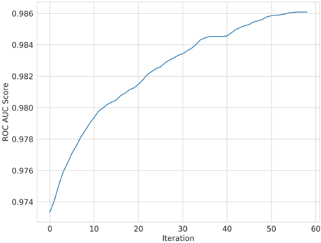
这样实现的贪心特征选择会返回得分和一个特征索引列表。图 2 展示了每轮迭代加入新特征后得分如何提升。我们看到,在某个点之后得分再也无法提高,而我们就在那里停下来。
另一种贪心方法叫做递归特征消除(recursive feature elimination,RFE)。在前一种方法中,我们从 1 个特征开始不断添加新特征;而在 RFE 中,我们从全部特征开始,每轮迭代移除一个对给定模型价值最小的特征。但我们怎么知道哪个特征提供的价值最小呢?如果我们使用线性支持向量机(support vector machine,SVM)或逻辑回归(logistic regression)这类模型,每个特征都会得到一个系数,它决定了特征的重要性。对于任何基于树的模型,我们得到的是特征重要性(feature importance),而不是系数。在每轮迭代中,我们可以剔除最不重要的特征,一直剔除到达到所需特征数量为止。所以,是的,我们能够决定要保留多少个特征。
图 2:贪心特征选择中 AUC 得分随新特征加入的变化
当我们做递归特征消除时,每轮迭代都移除特征重要性较低、或系数接近 0 的特征。请记住,当你使用逻辑回归这类模型做二分类时,对正类重要的特征系数更正,对负类重要的特征系数更负。把我们的贪心特征选择类稍加修改,就能创建一个用于递归特征消除的新类,不过 scikit-learn 也直接提供了 RFE。下面这个例子展示了它的简单用法。
import pandas as pd
from sklearn.feature_selection import RFE
from sklearn.linear_model import LinearRegression
from sklearn.datasets import fetch_california_housing

# fetch a regression dataset
data = fetch_california_housing()
X = data["data"]
col_names = data["feature_names"]
y = data["target"]

# initialize the model
model = LinearRegression()

# initialize RFE
rfe = RFE(
    estimator=model,
    n_features_to_select=3
)

# fit RFE
rfe.fit(X, y)

# selected columns
# get the transformed data with
X_transformed = rfe.transform(X)
我们看到了两种从模型中选特征的贪心方法。但你也可以把模型拟合到数据上,然后根据特征的系数或特征重要性从模型中选特征。如果使用系数,你可以设定一个阈值:系数高于该阈值就保留特征,否则就剔除。
让我们看看如何从随机森林(random forest)这类模型中获得特征重要性。
import pandas as pd
from sklearn.datasets import load_diabetes
from sklearn.ensemble import RandomForestRegressor

# fetch a regression dataset
# in diabetes data we predict diabetes progression
# after one year based on some features
data = load_diabetes()
X = data["data"]
col_names = data["feature_names"]
y = data["target"]

# initialize the model
model = RandomForestRegressor()

# fit the model
model.fit(X, y)
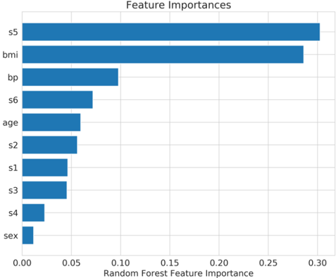
随机森林(或任何模型)的特征重要性可以这样绘制:
importances = model.feature_importances_
idxs = np.argsort(importances)
plt.title('Feature Importances')
plt.barh(range(len(idxs)), importances[idxs], align='center')
plt.yticks(range(len(idxs)), [col_names[i] for i in idxs])
plt.xlabel('Random Forest Feature Importance')
plt.show()
得到的图如图 3 所示。
图 3:特征重要性图
好吧,从模型中挑选最好的特征并不是什么新鲜事。你可以从一个模型中选特征,再用另一个模型来训练。例如,你可以用逻辑回归的系数来选特征,然后用随机森林在选出的特征上训练模型。Scikit-learn 还提供了 SelectFromModel 类,帮助你直接从给定模型中选择特征。你还可以按需指定系数或特征重要性的阈值,以及想要选择的最大特征数。
看看下面这段代码,我们用 SelectFromModel 的默认参数来选择特征。
import pandas as pd
from sklearn.datasets import load_diabetes
from sklearn.ensemble import RandomForestRegressor
from sklearn.feature_selection import SelectFromModel

# fetch a regression dataset
# in diabetes data we predict diabetes progression
# after one year based on some features
data = load_diabetes()
X = data["data"]
col_names = data["feature_names"]
y = data["target"]

# initialize the model
model = RandomForestRegressor()

# select from the model
sfm = SelectFromModel(estimator=model)
X_transformed = sfm.fit_transform(X, y)

# see which features were selected
support = sfm.get_support()

# get feature names
print([ x for x, y in zip(col_names, support) if y == True ])
它打印出:[‘bmi’, ‘s5’]。当我们看下图 3,会发现这正是最重要的前 2 个特征。因此,我们本也可以直接从随机森林提供的特征重要性中选取。这里我们还漏掉了一点:使用具有 L1(Lasso)惩罚的模型进行特征选择。当我们使用 L1 惩罚做正则化时,大部分系数都会是 0(或接近 0),我们选择系数非零的特征。只需把上面"从模型中选择"的代码片段里的随机森林替换成支持 L1 惩罚的模型(例如 lasso 回归)即可。所有基于树的模型都提供特征重要性,因此本章展示的所有基于模型的代码片段都可以用于 XGBoost、LightGBM 或 CatBoost。特征重要性的函数名可能不同,返回结果的格式也可能不同,但用法是一样的。最后,做特征选择时你必须小心。要在训练数据上选择特征,并在验证数据上验证模型,这样才能在不使模型过拟合的情况下正确选择特征。