特征工程
特征工程(feature engineering)是构建一个好的机器学习(machine learning)模型最关键的部分之一。如果我们拥有有用的特征,模型就会表现得更好。在很多情况下,你可以避开庞大而复杂的模型,转而使用带有精心设计特征的简单模型。我们必须记住:只有当你对问题所属领域有所了解时,特征工程才能以最佳方式完成,而且它在很大程度上取决于手头的数据。不过,也有一些通用技术,你可以尝试用它们从几乎所有类型的数值(numerical)变量和类别(categorical)变量中构造特征。特征工程不仅仅是从数据中创建新特征,还包括不同类型的归一化(normalization)和变换(transformation)。
在关于类别特征的章节中,我们已经看到了一种组合不同类别变量的方法,以及如何将类别变量转换为计数、目标编码(target encoding)和使用嵌入(embedding)。这些几乎就是从类别变量构造特征的所有方式。因此,在本章中,我们的重点将仅限于数值变量以及数值变量和类别变量的组合。
让我们从最简单但使用最广泛的特征工程技术开始。假设你正在处理日期和时间数据。于是我们有一个带日期时间(datetime)类型列的 pandas 数据框(DataFrame)。利用这一列,我们可以创建如下特征:
- 年份(year)
- 年中第几周(week of year)
- 月份(month)
- 星期几(day of week)
- 周末(weekend)
- 小时(hour)
- 以及更多。
使用 pandas 可以非常容易地完成这些操作。
df.loc[:, 'weekofyear'] = df['datetime_column'].dt.weekofyear
df.loc[:, 'year'] = df['datetime_column'].dt.year
df.loc[:, 'month'] = df['datetime_column'].dt.month
df.loc[:, 'dayofweek'] = df['datetime_column'].dt.dayofweek
df.loc[:, 'weekend'] = (df.datetime_column.dt.weekday >= 5).astype(int)
df.loc[:, 'hour'] = df['datetime_column'].dt.hour
于是,我们用日期时间列创建了一堆新列。下面来看一些可以创建的示例特征。
import pandas as pd
# create a series of datetime with a frequency of 10 hours
s = pd.date_range('2020-01-06', '2020-01-10', freq='10H').to_series()
# create some features based on datetime
features = {
    "dayofweek": s.dt.dayofweek.values,
    "dayofyear": s.dt.dayofyear.values,
    "hour": s.dt.hour.values,
    "is_leap_year": s.dt.is_leap_year.values,
    "quarter": s.dt.quarter.values,
    "weekofyear": s.dt.weekofyear.values
}
这将从给定的序列生成一个特征字典。你可以将其应用于 pandas 数据框中的任何日期时间列。这些只是 pandas 提供的众多日期时间特征中的一部分。当你处理时间序列(time series)数据时,日期时间特征至关重要,例如,预测一家商店的销售额,但又想对聚合(aggregated)特征使用 xgboost 之类的模型时。
假设我们有一个如下所示的数据框:
图 1:带有类别特征和日期特征的示例数据框
| date | customer_id | cat1 | cat2 | cat3 | num1 |
|---|---|---|---|---|---|
| 2016-09-01 | 146361 | 2 | 2 | 0 | -0.518679 |
| 2017-04-01 | 180838 | 4 | 1 | 0 | 0.415853 |
| 2017-08-01 | 157857 | 3 | 3 | 1 | -2.061687 |
| 2017-12-01 | 159772 | 5 | 1 | 1 | -0.276558 |
| 2017-09-01 | 80014 | 3 | 2 | 1 | -1.456827 |
在图 1 中,我们看到有一个日期(date)列,我们可以轻松地从中提取年份、月份、季度等特征。然后是一个 customer_id 列,其中包含多条记录,因此一个客户会出现多次(在截图里看不出来)。而每个日期和客户 ID 都附带三个类别特征和一个数值特征。我们可以从中创建一堆特征:
- 一个客户最活跃的月份是哪个月
- 一个客户在 cat1、cat2、cat3 上的计数是多少
- 在一年中的某个给定星期,一个客户的 cat1、cat2、cat3 计数是多少
- 某个给定客户的 num1 均值是多少
- 等等。
使用 pandas 中的聚合(aggregate),创建这样的特征相当容易。让我们看看怎么做。
def generate_features(df):
    # create a bunch of features using the date column
    df.loc[:, 'year'] = df['date'].dt.year
    df.loc[:, 'weekofyear'] = df['date'].dt.weekofyear
    df.loc[:, 'month'] = df['date'].dt.month
    df.loc[:, 'dayofweek'] = df['date'].dt.dayofweek
    df.loc[:, 'weekend'] = (df['date'].dt.weekday >= 5).astype(int)

    # create an aggregate dictionary
    aggs = {}
    # for aggregation by month, we calculate the
    # number of unique month values and also the mean
    aggs['month'] = ['nunique', 'mean']
    aggs['weekofyear'] = ['nunique', 'mean']
    # we aggregate by num1 and calculate sum, max, min
    # and mean values of this column
    aggs['num1'] = ['sum','max','min','mean']
    # for customer_id, we calculate the total count
    aggs['customer_id'] = ['size']
    # again for customer_id, we calculate the total unique
    aggs['customer_id'] = ['nunique']

    # we group by customer_id and calculate the aggregates
    agg_df = df.groupby('customer_id').agg(aggs)
    agg_df = agg_df.reset_index()
    return agg_df
请注意,在上面的函数中,我们跳过了类别变量,但你可以像使用其他聚合一样使用它们。
图 2:聚合特征及其他特征
| customer_id | month nunique | mean | weekofyear nunique mean | customer_id | size | sum | max | min | num1 mean |
|---|---|---|---|---|---|---|---|---|---|
| 0 | 1 | 2 | 1 | 5 | 1 | 0.134077 | 0.134077 | 0.134077 | 0.134077 |
| 1 | 1 | 7 | 1 | 26 | 1 | 0.884295 | 0.884295 | 0.884295 | 0.884295 |
| 2 | 1 | 9 | 1 | 35 | 1 | -0.264433 | -0.264433 | -0.264433 | -0.264433 |
| 3 | 1 | 5 | 1 | 18 | 1 | 0.812872 | 0.812872 | 0.812872 | 0.812872 |
| 4 | 1 | 4 | 1 | 13 | 1 | 1.288514 | 1.288514 | 1.288514 | 1.288514 |
| … | … | … | … | … | … | … | … | … | … |
| 201912 | 1 | 4 | 1 | 13 | 1 | 0.362965 | 0.362965 | 0.362965 | 0.362965 |
| 201913 | 1 | 11 | 1 | 44 | 1 | -0.085357 | -0.085357 | -0.085357 | -0.085357 |
| 201914 | 1 | 8 | 1 | 31 | 1 | 1.530061 | 1.530061 | 1.530061 | 1.530061 |
| 201915 | 1 | 1 | 1 | 1 | 1 | -0.600063 | -0.600063 | -0.600063 | -0.600063 |
| 201916 | 1 | 8 | 1 | 31 | 1 | -1.073077 | -1.073077 | -1.073077 | -1.073077 |
现在,我们可以把图 2 中的这个数据框与带有 customer_id 列的原始数据框连接起来,开始训练模型。这里我们并不试图预测什么,只是创建通用特征。不过,如果我们在这里试图预测什么,创建特征会更容易。
有时,例如在处理时间序列问题时,你可能会遇到一些特征,它们不是单个值,而是一列值。例如,一个客户在给定时间段内的交易。在这些情况下,我们会创建不同类型的特征,例如:对于数值特征,当你按某个类别列分组时,你会得到一列随时间分布的值。在这些情况下,你可以创建一堆统计(statistical)特征,例如:
- 均值(mean)
- 最大值(max)
- 最小值(min)
- 唯一值(unique)
- 偏度(skewness)
- 峰度(kurtosis)
- K 统计量(kstat)
- 百分位数(percentile)
- 分位数(quantile)
- 峰峰值(peak to peak)
- 以及更多
这些可以使用简单的 numpy 函数创建,如下面的 Python 代码片段所示。
import numpy as np
feature_dict = {}
# calculate mean
feature_dict['mean'] = np.mean(x)
# calculate max
feature_dict['max'] = np.max(x)
# calculate min
feature_dict['min'] = np.min(x)
# calculate standard deviation
feature_dict['std'] = np.std(x)
# calculate variance
feature_dict['var'] = np.var(x)
# peak-to-peak
feature_dict['ptp'] = np.ptp(x)
# percentile features
feature_dict['percentile_10'] = np.percentile(x, 10)
feature_dict['percentile_60'] = np.percentile(x, 60)
feature_dict['percentile_90'] = np.percentile(x, 90)
# quantile features
feature_dict['quantile_5'] = np.quantile(x, 0.05)
feature_dict['quantile_95'] = np.quantile(x, 0.95)
feature_dict['quantile_99'] = np.quantile(x, 0.99)
时间序列数据(一列值)可以转换成大量特征。
一个名为 tsfresh 的 Python 库在这种情况下非常有用。
from tsfresh.feature_extraction import feature_calculators as fc
# tsfresh based features
feature_dict['abs_energy'] = fc.abs_energy(x)
feature_dict['count_above_mean'] = fc.count_above_mean(x)
feature_dict['count_below_mean'] = fc.count_below_mean(x)
feature_dict['mean_abs_change'] = fc.mean_abs_change(x)
feature_dict['mean_change'] = fc.mean_change(x)
这还不是全部;tsfresh 提供了数百种特征以及数十种不同特征的变体,你可以将它们用于基于时间序列(一列值)的特征。在上面的示例中,x 是一列值。但这还不是全部。对于数值数据(无论是否带有类别数据),你还可以创建许多其他特征。生成大量特征的一个简单方法就是创建一堆多项式(polynomial)特征。例如,由两个特征 \(a\) 和 \(b\) 生成的二次多项式特征将包括:\(a\)、\(b\)、\(ab\)、\(a^2\) 和 \(b^2\)。
import numpy as np
# generate a random dataframe with
# 2 columns and 100 rows
df = pd.DataFrame(
    np.random.rand(100, 2),
    columns=[f"f_{i}" for i in range(1, 3)]
)
这样就得到一个如图 3 所示的数据框。
图 3:包含两个数值特征的随机数据框
| f_1 | f_2 |
|---|---|
| 0.118305 | 0.648567 |
| 0.503417 | 0.117854 |
| 0.067735 | 0.158106 |
| 0.907574 | 0.436235 |
| 0.134100 | 0.824813 |
我们可以使用 scikit-learn 中的 PolynomialFeatures 创建二次多项式特征。
from sklearn import preprocessing
# initialize polynomial features class object
# for two-degree polynomial features
pf = preprocessing.PolynomialFeatures(
    degree=2,
    interaction_only=False,
    include_bias=False
)
# fit to the features
pf.fit(df)
# create polynomial features
poly_feats = pf.transform(df)
# create a dataframe with all the features
num_feats = poly_feats.shape[1]
df_transformed = pd.DataFrame(
    poly_feats,
    columns=[f"f_{i}" for i in range(1, num_feats + 1)]
)
这会得到一个如图 4 所示的数据框。
图 4:包含多项式特征的示例数据框
| f_1 | f_2 | f_3 | f_4 | f_5 |
|---|---|---|---|---|
| 0.118305 | 0.648567 | 0.013996 | 0.0767290 | 0.420639 |
| 0.503417 | 0.117854 | 0.253429 | 0.059330 | 0.013890 |
| 0.067735 | 0.158106 | 0.004588 | 0.010709 | 0.024997 |
| 0.907574 | 0.436235 | 0.823691 | 0.395916 | 0.190301 |
| 0.134100 | 0.824813 | 0.017983 | 0.110608 | 0.680317 |
这样,我们现在已经创建了一些多项式特征。如果你创建三次多项式特征,最终会得到总共九个特征。特征的数量越多,多项式特征的数量就越多,而且你还必须记住,如果数据集中的样本很多,创建这类特征会花费一些时间。
value
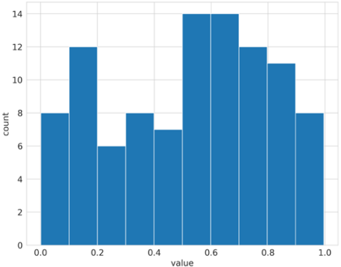
图 5:数值特征列的直方图
另一个有趣的技巧是把数字转换为类别,它被称为分箱(binning)。让我们看一下图 5,它展示了一个随机数值特征的示例直方图。这张图用了十个箱(bin),我们可以看到可以把数据分成十部分。这可以通过 pandas 的 cut 函数来完成。
# create bins of the numerical columns
# 10 bins
df["f_bin_10"] = pd.cut(df["f_1"], bins=10, labels=False)
# 100 bins
df["f_bin_100"] = pd.cut(df["f_1"], bins=100, labels=False)
这会在数据框中生成两个新特征,如图 6 所示。
图 6:数值特征分箱
| f_1 | f_2 | f_bin_10 | f_bin_100 |
|---|---|---|---|
| 0.143246 | 0.286327 | 1 | 12 |
| 0.421268 | 0.967212 | 4 | 41 |
| 0.224104 | 0.075204 | 2 | 21 |
| 0.859183 | 0.651964 | 8 | 86 |
| 0.082291 | 0.669589 | 0 | 6 |
分箱时,你可以同时使用分箱结果和原始特征。本章后面我们会进一步了解特征选择。分箱还使你能够把数值特征当作类别特征来对待。
另一种可以从数值特征中创建的有趣特征是对数变换(log transformation)。看一下图 7 中的特征 f_3。
图 7:高方差特征的示例
| f_1 | f_2 | f_bin_10 | f_bin_100 | f_3 |
|---|---|---|---|---|
| 0.143246 | 0.286327 | 1 | 12 | 8048 |
| 0.421268 | 0.967212 | 4 | 41 | 7433 |
| 0.224104 | 0.075204 | 2 | 21 | 2289 |
| 0.859183 | 0.651964 | 8 | 86 | 1153 |
| 0.082291 | 0.669589 | 0 | 6 | 2201 |
f_3 是一个方差(variance)非常高的特殊特征,而其他特征的方差都很低(我们这样假设)。因此,我们希望降低这一列的方差,这可以通过对数变换来实现。
列 f_3 中的值范围从 0 到 10000,其直方图如图 8 所示。
图 8:特征 f_3 的直方图
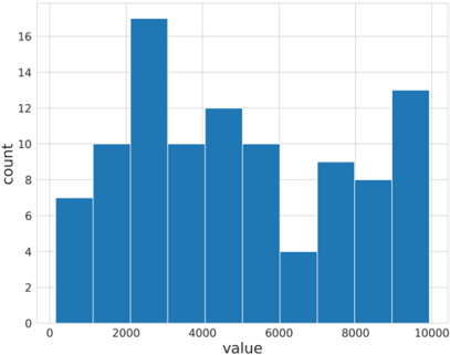
我们可以对这一列应用 \(\log(1 + x)\) 来降低其方差。图 9 展示了应用对数变换后直方图发生的变化。
图 9:应用对数变换后特征 f_3 的直方图
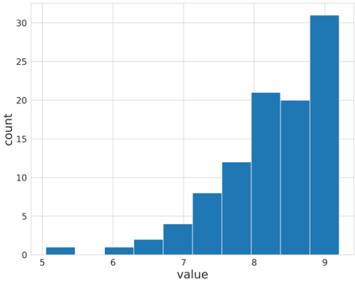
让我们看一下应用对数变换前后的方差。
In [X]: df.f_3.var()
Out[X]: 8077265.875858586

In [X]: df.f_3.apply(lambda x: np.log(1 + x)).var()
Out[X]: 0.6058771732119975
有时,除了对数,你也可以使用指数(exponential)。一个非常有趣的情况是当你使用基于对数的评估指标时,例如 RMSLE。在这种情况下,你可以在对数变换后的目标值上训练模型,然后在预测结果上使用指数变换转换回原始值。这将有助于针对该指标优化模型。
大多数时候,这类数值特征是基于直觉创建的。没有固定的公式。如果你在某个行业工作,你会创建行业特有的特征。
当同时处理类别变量和数值变量时,你可能会遇到缺失值(missing values)。在上一章中,我们看到了处理类别特征中缺失值的一些方法,但处理缺失值/NaN 的方法还有很多。这同样被视为特征工程。
对于类别特征,让我们保持超级简单。如果你在类别特征中遇到缺失值,就把它当作一个新类别!尽管方法如此简单,它(几乎)总是有效的!
填充数值数据中缺失值的一种方法是选择一个在该特定特征中不出现的值,并用它来填充。例如,假设特征中没有出现 0,我们就用 0 填充所有缺失值。这是其中一种方法,但可能不是最有效的。对于数值数据,比填充 0 效果更好的方法之一是改用均值填充。你也可以尝试用该特征所有值的中位数填充,或者用最常见的值来填充缺失值。方法实在太多了。
一种更花哨的缺失值填充方法是使用 K 近邻(K-nearest neighbors, KNN)方法。你可以选择一个有缺失值的样本,利用某种距离度量(例如欧氏距离(Euclidean distance))找到最近的邻居。然后取所有最近邻居的均值来填充缺失值。你可以使用 KNN 插补器(KNNImputer)的实现来这样填充缺失值。
图 10:带缺失值的二维数组
[ 4., nan, 10., nan, 10., 11.]
[14.,  2., 14.,  6., 10., 14.]
[ 6., 12.,  8.,  6.,  2.]
[nan, 14., nan,  1.,  2.,  5.]
[ 1.,  7.,  6., 13., 14.,  9.]
[10.,  2., 14., nan, nan,  1.]
[ 3., 14.,  3.,  7., 13.,  9.]
[11., nan,  1., nan,  4.,  7.]
[ 4.,  8.,  2.,  2.,  6., nan]
[ 2., nan, 13.,  9.,
让我们看看 KNNImputer 如何处理如图 10 所示的带缺失值的矩阵。
import numpy as np
from sklearn import impute
# create a random numpy array with 10 samples
# and 6 features and values ranging from 1 to 15
X = np.random.randint(1, 15, (10, 6))
# convert the array to float
X = X.astype(float)
# randomly assign 10 elements to NaN (missing)
# use 2 nearest neighbours to fill na values
knn_imputer = impute.KNNImputer(n_neighbors=2)
knn_imputer.fit_transform(X)
X.ravel()[np.random.choice(X.size, 10, replace=False)] = np.nan
它会填充上面的矩阵,如图 11 所示。
图 11:由 KNN 插补器插补后的数值
[ 4. , 10.5, 10. , 10. , 10. , 11. ]
[14. ,  2. , 14. ,  6. , 10. , 14. ]
[ 7. ,  6. , 12. ,  8. ,  6. ,  2. ]
[ 7.5, 14. ,  1.5,  1. ,  2. ,  5. ]
[ 1. ,  7. ,  6. , 13. , 14. ,  9. ]
[10. ,  2. , 14. ,  7. ,  8. ,  1. ]
[ 3. , 14. ,  3. ,  7. , 13. ,  9. ]
[11. , 11. ,  1. ,  1.5,  4. ,  7. ]
[ 4. ,  8. ,  2. ,  2. ,  6. ,  6. ]
在某一列中插补缺失值的另一种方法是训练一个回归(regression)模型,尝试根据其他列来预测该列中的缺失值。因此,你从一列有缺失值的列开始,把这一列当作回归模型的目标列(不包括缺失值)。利用所有其他列,你现在在那些相关列中没有缺失值的样本上训练模型,然后尝试为之前剔除的样本预测目标值(即同一列)。这样,你就有了一个更稳健的基于模型的插补(imputation)。
永远记住:对于基于树的(tree-based)模型,插补是不必要的,因为它们自己就能处理。
到目前为止,我所展示的只是创建特征的一些通用方法。现在,假设你在做一个预测不同商品门店销售额(按周或按月)的问题。你有商品,也有门店 ID。因此,你可以创建诸如每家门店的商品数量之类的特征。这种特征就是前面没有讨论过的类型。这类特征无法泛化,完全来自领域、数据和业务知识。观察数据,看看什么合适,然后相应地创建特征。并且永远记住:如果你使用逻辑回归(logistic regression)之类的线性模型或 SVM 之类的模型,一定要对特征进行缩放(scaling)或归一化。基于树的模型在没有任何特征归一化的情况下也总能正常工作。