处理类别变量
很多人都对类别变量(categorical variables)的处理感到非常棘手,因此这值得用一整章来讲解。在本章中,我将讨论不同类型的类别数据,以及如何着手解决包含类别变量的问题。
什么是类别变量?
类别变量/特征可以分为两大类型:
- 名义变量(Nominal)
- 有序变量(Ordinal)
名义变量是指具有两个或更多类别、且这些类别之间没有任何顺序关系的变量。例如,如果性别被分为两组,即男性和女性,那么它就可以被视为名义变量。
另一方面,有序变量具有与之相关联的特定顺序的「水平」或类别。例如,一个有序类别变量可以是一个具有三个不同水平的特征:低(low)、中(medium)和高(high)。顺序很重要。
就定义而言,我们还可以把类别变量划分为二元(binary)变量,即只有两个类别的类别变量。有些人还会谈到一种叫做「循环(cyclic)」的类别变量类型。循环变量以「循环」的形式存在,例如一周中的几天:周日、周一、周二、周三、周四、周五和周六。周六之后,我们又迎来周日。这就是一个循环。另一个例子是如果把一天中的小时视为类别,那么它也是循环的。
关于类别变量有很多不同的定义,也有很多人根据类别变量的类型来讨论不同的处理方法。然而,我认为没有必要这样做。所有包含类别变量的问题都可以用同样的方式处理。
在我们开始之前,需要一个数据集来动手实践(一如既往)。理解类别变量的最佳免费数据集之一,是来自 Kaggle 上 Categorical Features Encoding Challenge(类别特征编码挑战赛)的 cat-in-the-dat 数据集。这个挑战赛有两届,我们将使用第二届的数据,因为它的变量更多,也比上一届更难。
让我们看一下数据
图 1:查看数据的一个子集。Cat-in-the-dat-ii 挑战⁵
| bin_0 | bin_1 | nom_0 | nom_1 | ord_0 | ord_1 | day | month | target |
|---|---|---|---|---|---|---|---|---|
| NaN | 0.0 | Green | Polygon | 3.0 | Novice | 6.0 | 8.0 | 0 |
| 0.0 | 0.0 | Red | Square | 1.0 | Expert | 7.0 | 1.0 | 0 |
| 0.0 | 0.0 | Blue | Trapezoid | 1.0 | Expert | 5.0 | 8.0 | 0 |
| 0.0 | 0.0 | Green | Circle | 1.0 | Contributor | 3.0 | 6.0 | 0 |
| 0.0 | 0.0 | Blue | Circle | 1.0 | Expert | 2.0 | 4.0 | 0 |
| … | … | … | … | … | … | … | … | |
| 0.0 | 0.0 | Red | Triangle | 2.0 | Expert | 3.0 | 11.0 | 1 |
| 0.0 | 1.0 | Blue | Circle | 3.0 | Novice | 4.0 | 5.0 | 0 |
| 0.0 | 0.0 | Red | Polygon | 3.0 | Grandmaster | 1.0 | 8.0 | 0 |
| 1.0 | 1.0 | Blue | Trapezoid | 2.0 | Novice | 7.0 | 5.0 | 0 |
| 0.0 | 1.0 | Red | Circle | 1.0 | Novice | 2.0 | 11.0 | 0 |
该数据集包含各种各样的类别变量:
- 名义变量(Nominal)
- 有序变量(Ordinal)
- 循环变量(Cyclical)
- 二元变量(Binary)
在图 1 中,我们只看到了所有变量中的一部分,以及目标变量。
这是一个二分类(binary classification)问题。
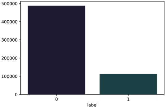
目标变量对我们学习类别变量来说并不是那么重要,但最后我们还是要构建一个端到端(end-to-end)的模型,所以让我们看一下图 2 中的目标分布。可以看到目标是有偏(skewed)的,因此这个二分类问题的最佳评估指标是 ROC 曲线下面积(Area Under the ROC Curve,AUC)。我们也可以使用精确率(precision)和召回率(recall),但 AUC 综合了这两个指标。因此,我们将使用 AUC 来评估我们在这个数据集上构建的模型。
5 https://www.kaggle.com/c/cat-in-the-dat-ii
图 2:目标的计数。x 轴显示标签,y 轴显示标签的计数
总体而言,数据集中有:
- 五个二元变量
- 十个名义变量
- 六个有序变量
- 两个循环变量
- 以及一个目标变量
让我们看看数据集中的 ord_2 特征,它包含六个不同的类别:
- Freezing
- Warm
- Cold
- Boiling Hot
- Hot
- Lava Hot
我们必须知道,计算机不理解文本数据,因此我们需要把这些类别转换为数字。一个简单的做法是创建一个字典,将这些值映射为从 0 到 N-1 的数字,其中 N 是给定特征中类别的总数。
mapping = { "Freezing": 0, "Warm": 1, "Cold": 2, "Boiling Hot": 3, "Hot": 4, "Lava Hot": 5 }
现在,我们可以读取数据集,轻松地将这些类别转换为数字。
import pandas as pd
df = pd.read_csv("../input/cat_train.csv")
df.loc[:, "ord_2"] = df.ord_2.map(mapping)
映射前的值计数:
df.ord_2.value_counts()
Freezing       142726
Warm           124239
Cold            97822
Boiling Hot     84790
Hot             67508
Lava Hot        64840
Name: ord_2, dtype: int64
映射后的值计数:
0.0    142726
1.0    124239
2.0     97822
3.0     84790
4.0     67508
5.0     64840
Name: ord_2, dtype: int64
这种类别变量编码方式被称为标签编码(label encoding),即我们把每个类别编码为一个数字标签。
我们也可以用 scikit-learn 的 LabelEncoder 做同样的事情。
import pandas as pd
from sklearn import preprocessing
# read the data
df = pd.read_csv("../input/cat_train.csv")
# fill NaN values in ord_2 column
df.loc[:, "ord_2"] = df.ord_2.fillna("NONE")
# initialize LabelEncoder
lbl_enc = preprocessing.LabelEncoder()
# fit label encoder and transform values on ord_2 column
# P.S: do not use this directly. fit first, then transform
df.loc[:, "ord_2"] = lbl_enc.fit_transform(df.ord_2.values)
你会看到我使用了 pandas 的 fillna。原因是 scikit-learn 的 LabelEncoder 不处理 NaN 值,而 ord_2 列中包含 NaN 值。
我们可以直接在许多基于树的模型(tree-based models)中使用这种编码:
- 决策树(Decision trees)
- 随机森林(Random forest)
- 极端随机树(Extra Trees)
- 或任何一种提升树模型(boosted trees model)
- XGBoost
- GBM
- LightGBM
这种编码不能用于线性模型(linear models)、支持向量机(support vector machines)或神经网络(neural networks),因为它们期望数据是归一化(normalized,或标准化 standardized)的。
对于这类模型,我们可以对数据进行二值化(binarize)。
| 类别 | 标签编码 | 二进制表示 |
|---|---|---|
| Freezing | 0 | 0 0 0 |
| Warm | 1 | 0 0 1 |
| Cold | 2 | 0 1 0 |
| Boiling Hot | 3 | 0 1 1 |
| Hot | 4 | 1 0 0 |
| Lava Hot | 5 | 1 0 1 |
这只是先把类别转换为数字,再把它们转换为二进制表示。因此,我们实际上是把一个特征拆分成了三个(在这个例子中)特征(或列)。如果我们有更多的类别,最终可能会拆分成多得多的列。
如果我们以稀疏格式(sparse format)存储,就可以很容易地存储大量这样的二值化变量。稀疏格式不过是一种在内存中表示或存储数据的方式:你不存储所有的值,只存储那些重要的值。在上述二元变量的例子中,重要的只是那些为 1 的位置。
这种格式很难凭空想象,但通过一个例子应该就能明白了。
假设上面的数据框中只给我们提供了一个特征:ord_2。
| 索引 | 特征 |
|---|---|
| 0 | Warm |
| 1 | Hot |
| 2 | Lava hot |
目前我们只看数据集中的三个样本。让我们把它转换为二进制表示,每个样本对应三个项。
这三个项就是三个特征。
| 索引 | 特征_0 | 特征_1 | 特征_2 |
|---|---|---|---|
| 0 | 0 | 0 | 1 |
| 1 | 1 | 0 | 0 |
| 2 | 1 | 0 | 1 |
所以,我们的特征存储在一个 3 行 3 列的矩阵中——3x3。这个矩阵的每个元素占 8 字节。因此,这个数组的总内存需求是 8x3x3 = 72 字节。
我们也可以用一段简单的 python 代码来验证。
import numpy as np
# create our example feature matrix
example = np.array( [ [0, 0, 1], [1, 0, 0], [1, 0, 1] ] )
# print size in bytes
print(example.nbytes)
这段代码会像我们之前计算的那样打印出 72。但我们真的需要存储这个矩阵的所有元素吗?不需要。如前所述,我们只关心 1。0 并不那么重要,因为任何数乘以 0 都是 0,任何数加/减 0 都不会有任何变化。只用 1 来表示这个矩阵的一种方法是某种字典方法,其中键是行和列的索引,值是 1:
(0, 2) 1
(1, 0) 1
(2, 0) 1
(2, 2) 1
这样的表示法占用的内存要少得多,因为它只需要存储四个值(在这个例子中)。总内存占用将是 8x4 = 32 字节。任何 numpy 数组都可以用简单的 python 代码转换为稀疏矩阵。
import numpy as np
from scipy import sparse
# create our example feature matrix
example = np.array( [ [0, 0, 1], [1, 0, 0], [1, 0, 1] ] )
# convert numpy array to sparse CSR matrix
sparse_example = sparse.csr_matrix(example)
# print size of this sparse matrix
print(sparse_example.data.nbytes)
这会打印出 32,比我们的稠密数组小太多了!稀疏 csr 矩阵的总大小是三个值的和。
print( sparse_example.data.nbytes + sparse_example.indptr.nbytes + sparse_example.indices.nbytes )
这会打印出 64,仍然小于我们的稠密数组。遗憾的是,我不会深入讲解这些元素的细节。你可以在 scipy 文档中了解更多。当我们有更大的数组时,比如数千个样本、数万个特征,这种大小差异就会变得非常巨大。例如,使用基于计数的特征(count-based features)的文本数据集。
import numpy as np
from scipy import sparse
# number of rows
n_rows = 10000
# number of columns
n_cols = 100000
# create random binary matrix with only 5% values as 1s
example = np.random.binomial(1, p=0.05, size=(n_rows, n_cols))
# print size in bytes
print(f"Size of dense array: {example.nbytes}")
# convert numpy array to sparse CSR matrix
sparse_example = sparse.csr_matrix(example)
# print size of this sparse matrix
print(f"Size of sparse array: {sparse_example.data.nbytes}")
full_size = ( sparse_example.data.nbytes + sparse_example.indptr.nbytes + sparse_example.indices.nbytes )
# print full size of this sparse matrix
print(f"Full size of sparse array: {full_size}")
这会打印:
Size of dense array: 8000000000
Size of sparse array: 399932496
Full size of sparse array: 599938748
所以,稠密数组大约占用 8000MB,即约 8GB 内存。而稀疏数组只占用 399MB 内存。
这就是为什么只要特征中有大量 0,我们就会优先选择稀疏数组而不是稠密数组。
请注意,表示稀疏矩阵的方法有很多种。这里我只展示了一种(可能也是最流行的一种)。深入探讨这些内容超出了本书的范围,留给读者作为练习。
尽管二值化特征的稀疏表示比其稠密表示占用的内存少得多,但还有另一种类别变量的转换方式,占用的内存更少。这就是众所周知的独热编码(one-hot encoding)。
从只有 0 和 1 两个值这个意义上说,独热编码也是一种二元编码。但必须注意,它不是二进制表示。它的表示方式可以通过下面的例子来理解。
假设我们用向量来表示 ord_2 变量的每个类别。这个向量的大小与 ord_2 变量中的类别数量相同。在这个具体例子中,每个向量的大小都是 6,除一个位置外全部为 0。让我们看一下这个向量表。
| Freezing | 0 | 0 | 0 | 0 | 0 | 1 |
|---|---|---|---|---|---|---|
| Warm | 0 | 0 | 0 | 0 | 1 | 0 |
| Cold | 0 | 0 | 0 | 1 | 0 | 0 |
| Boiling Hot | 0 | 0 | 1 | 0 | 0 | 0 |
| Hot | 0 | 1 | 0 | 0 | 0 | 0 |
| Lava Hot | 1 | 0 | 0 | 0 | 0 | 0 |
我们看到向量的大小是 1x6,即向量中有六个元素。这个数字从何而来?如果你仔细看,会发现正如前面提到的,这里有六个类别。做独热编码时,向量的大小必须与我们面对的类别数量相同。每个向量有一个 1,其余所有值都是 0。现在,让我们用这些特征代替之前的二值化特征,看看能省下多少内存。
如果你还记得旧数据,它长这样:
| 索引 | 特征 |
|---|---|
| 0 | Warm |
| 1 | Hot |
| 2 | Lava hot |
之前每个样本有三个特征。但在这个例子中,独热向量的大小是 6。因此,我们有六个特征而不是三个。
| 索引 | F_0 | F_1 | F_2 | F_3 | F_4 | F_5 |
|---|---|---|---|---|---|---|
| 0 | 0 | 0 | 0 | 0 | 1 | 0 |
| 1 | 0 | 1 | 0 | 0 | 0 | 0 |
| 2 | 1 | 0 | 0 | 0 | 0 | 0 |
所以,我们有六个特征,在这个 3x6 数组中只有 3 个 1。用 numpy 计算大小与二值化的大小计算脚本非常相似。你只需要更换数组。让我们看一下这段代码。
import numpy as np
from scipy import sparse
# create binary matrix
example = np.array( [ [0, 0, 0, 0, 1, 0], [0, 1, 0, 0, 0, 0], [1, 0, 0, 0, 0, 0] ] )
# print size in bytes
print(f"Size of dense array: {example.nbytes}")
# convert numpy array to sparse CSR matrix
sparse_example = sparse.csr_matrix(example)
# print size of this sparse matrix
print(f"Size of sparse array: {sparse_example.data.nbytes}")
full_size = ( sparse_example.data.nbytes + sparse_example.indptr.nbytes + sparse_example.indices.nbytes )
# print full size of this sparse matrix
print(f"Full size of sparse array: {full_size}")
This will print the sizes as:
Size of dense array: 144
Size of sparse array: 24
Full size of sparse array: 52
我们看到稠密数组的大小比二值化时大得多。然而,稀疏数组的大小则小得多。让我们用一个更大的数组来试试。在这个例子中,我们将使用 scikit-learn 的 OneHotEncoder,把包含 1001 个类别的特征数组转换为稠密矩阵和稀疏矩阵。
import numpy as np
from sklearn import preprocessing
# create random 1-d array with 1001 different categories (int)
example = np.random.randint(1000, size=1000000)
# initialize OneHotEncoder from scikit-learn
# keep sparse = False to get dense array
ohe = preprocessing.OneHotEncoder(sparse=False)
# fit and transform data with dense one hot encoder
ohe_example = ohe.fit_transform(example.reshape(-1, 1))
# print size in bytes for dense array
print(f"Size of dense array: {ohe_example.nbytes}")
# initialize OneHotEncoder from scikit-learn
# keep sparse = True to get sparse array
ohe = preprocessing.OneHotEncoder(sparse=True)
# fit and transform data with sparse one-hot encoder
ohe_example = ohe.fit_transform(example.reshape(-1, 1))
# print size of this sparse matrix
print(f"Size of sparse array: {ohe_example.data.nbytes}")
full_size = ( ohe_example.data.nbytes + ohe_example.indptr.nbytes + ohe_example.indices.nbytes )
# print full size of this sparse matrix
print(f"Full size of sparse array: {full_size}")
而这段代码会打印:
Size of dense array: 8000000000
Size of sparse array: 8000000
Full size of sparse array: 16000004
这里的稠密数组大小约为 8GB,而稀疏数组是 8MB。如果让你选择,你会选哪个?对我来说,这似乎是个相当简单的选择,不是吗?
这三种方法是处理类别变量最重要的方式。不过,你还可以使用许多其他不同的方法。其中一种方法就是把类别变量转换为数值变量。
假设我们回到之前看到的类别特征数据框(原始的 cat-in-the-dat-ii)。数据框中 ord_2 的值为 Boiling Hot 的有多少行 id?
我们可以通过计算 ord_2 列取值为 Boiling Hot 的数据框的 shape 来轻松得到这个值。
In [X]: df[df.ord_2 == "Boiling Hot"].shape
Out[X]: (84790, 25)
我们看到有 84790 行是这个值。我们也可以用 pandas 的 groupby 计算所有类别的这个值。
In [X]: df.groupby(["ord_2"])["id"].count()
Out[X]: ord_2
Boiling Hot     84790
Cold            97822
Freezing       142726
Hot             67508
Lava Hot        64840
Warm           124239
Name: id, dtype: int64
如果我们直接用它的计数值替换 ord_2 列,就把它转换成了一个有点数值化的特征。我们可以使用 pandas 的 transform 函数配合 groupby 来创建新列或替换这一列。
In [X]: df.groupby(["ord_2"])["id"].transform("count")
Out[X]: 0          67508.0
1         124239.0
2         142726.0
3          64840.0
4          97822.0
...
599995    142726.0
599996     84790.0
599997    142726.0
599998    124239.0
599999     84790.0
Name: id, Length: 600000, dtype: float64
你可以把所有特征的计数都加上,也可以替换它们,还可以按多列分组并计算它们的计数。例如,下面的代码按 ord_1 和 ord_2 列分组计数。
In [X]: df.groupby(
...:     [
...:         "ord_1",
...:         "ord_2"
...:     ]
...: )["id"].count().reset_index(name="count")
Out[X]: ord_1        ord_2  count
0   Contributor  Boiling Hot  15634
1   Contributor         Cold  17734
2   Contributor     Freezing  26082
3   Contributor          Hot  12428
4   Contributor     Lava Hot  11919
5   Contributor         Warm  22774
6        Expert  Boiling Hot  19477
7        Expert         Cold  22956
8        Expert     Freezing  33249
9        Expert          Hot  15792
10       Expert     Lava Hot  15078
11       Expert         Warm  28900
12  Grandmaster  Boiling Hot  13623
13  Grandmaster         Cold  15464
14  Grandmaster     Freezing  22818
15  Grandmaster          Hot  10805
16  Grandmaster     Lava Hot  10363
17  Grandmaster         Warm  19899
18       Master  Boiling Hot  10800
. . . .
请注意,为了让输出能放在一页里,我省略了一些行。这是另一种可以作为特征加入的计数。你肯定已经注意到,我一直在用 id 列做计数。不过,你也可以通过列的组合分组来统计其他列。
另一个技巧是从这些类别变量中创建新特征。你可以从现有特征中创建新的类别特征,而且做起来毫不费力。
In [X]: df["new_feature"] = (
...:     df.ord_1.astype(str)
...:     + "_"
...:     + df.ord_2.astype(str)
...: )
In [X]: df.new_feature
Out[X]: 0                 Contributor_Hot
1                Grandmaster_Warm
2                    nan_Freezing
3                 Novice_Lava Hot
4                Grandmaster_Cold
...
599995            Novice_Freezing
599996         Novice_Boiling Hot
599997       Contributor_Freezing
599998                Master_Warm
599999    Contributor_Boiling Hot
Name: new_feature, Length: 600000, dtype: object
这里,我们用下划线把 ord_1 和 ord_2 组合起来,在此之前,我们先把这些列转换为字符串类型。注意,NaN 也会转换为字符串。但这没关系。我们也可以把 NaN 当作一个新类别。这样,我们就有了一个新特征,它是这两个特征的组合。你还可以组合三个、四个甚至更多的列。
In [X]: df["new_feature"] = (
...:     df.ord_1.astype(str)
...:     + "_"
...:     + df.ord_2.astype(str)
...:     + "_"
...:     + df.ord_3.astype(str)
...: )
In [X]: df.new_feature
Out[X]: 0                 Contributor_Hot_c
1                Grandmaster_Warm_e
2                    nan_Freezing_n
3                 Novice_Lava Hot_a
4                Grandmaster_Cold_h
...
599995            Novice_Freezing_a
599996         Novice_Boiling Hot_n
599997       Contributor_Freezing_n
599998                Master_Warm_m
599999    Contributor_Boiling Hot_b
Name: new_feature, Length: 600000, dtype: object
那么应该组合哪些类别呢?这个问题没有简单的答案。这取决于你的数据和特征类型。创建这样的特征时,一些领域知识可能会很有用。但如果你不担心内存和 CPU 占用,可以采用贪心(greedy)的做法:创建许多这样的组合,然后用模型来决定哪些特征有用并保留它们。我们会在本书后面讲到这一点。
每当你遇到类别变量时,遵循以下简单步骤:
- 填充 NaN 值(这非常重要!)
- 使用 scikit-learn 的 LabelEncoder 或映射字典应用标签编码,将它们转换为整数。如果你没有用某个值填充 NaN,可能需要在这一步处理它们
- 创建独热编码。是的,你可以跳过二值化!
- 然后开始建模!我指的是机器学习建模,而不是上跑道(on the ramp)的那种。
处理类别特征中的 NaN 数据非常必要,否则你可能会遇到 scikit-learn 的 LabelEncoder 那个臭名昭著的错误:
ValueError: y contains previously unseen labels: [nan, nan, nan, nan, nan, nan, nan, nan]
这仅仅意味着当你在转换测试数据时,里面有 NaN 值。这是因为你在训练时忘了处理它们。处理 NaN 值的一个简单方法是把它们丢弃。嗯,这很简单,但并不理想。NaN 值中可能包含大量信息,如果你直接丢弃这些值,就会丢失这些信息。在很多情况下,你的大部分数据都是 NaN 值,因此你不能丢弃带有 NaN 值的行/样本。另一种处理 NaN 值的方法是把它们当作一个全新的类别。这是最受推崇的处理 NaN 值的方法。如果你使用 pandas,实现起来非常简单。
看看我们一直看到的这份数据中的 ord_2 列。
In [X]: df.ord_2.value_counts()
Out[X]: Freezing       142726
Warm           124239
Cold            97822
Boiling Hot     84790
Hot             67508
Lava Hot        64840
Name: ord_2, dtype: int64
填充 NaN 值之后,它变成:
In [X]: df.ord_2.fillna("NONE").value_counts()
Out[X]: Freezing       142726
Warm           124239
Cold            97822
Boiling Hot     84790
Hot             67508
Lava Hot        64840
NONE            18075
Name: ord_2, dtype: int64
哇!这一列中有 18075 个 NaN 值,我们之前甚至没有考虑过它们。随着这个新类别的加入,类别总数从 6 增加到了 7。这没关系,因为现在我们构建模型时也会把 NaN 考虑进去。我们拥有的相关信息越多,模型就越好。
假设 ord_2 没有任何 NaN 值。我们看到这一列中所有类别都有可观的计数。没有「稀有(rare)」类别,即只占样本总数很小百分比的类别。现在,假设你已经在生产环境中部署了这个使用该列的模型,当模型或项目上线后,你在 ord_2 列中得到了一个训练集中不存在的类别。在这种情况下,你的模型管道会抛出错误,而你对此无能为力。如果发生这种情况,那很可能是你的生产管道出了问题。如果这种情况是预期内的,那么你必须修改模型管道,把新类别加入这六个类别中。
这个新类别被称为「稀有」类别。稀有类别是一种不常出现的类别,它可以包含许多不同的类别。你也可以尝试用最近邻(nearest neighbour)模型来「预测」未知类别。记住,如果你预测了这个类别,它就会变成训练数据中的类别之一。
图 3:一个包含不同特征、没有目标的数据集示意图,其中一个特征在测试集或线上数据中出现时可能取到新值
| 假设这个特征在测试/线上阶段可能出现新值 | 假设这个特征在测试/线上阶段可能出现新值 | 假设这个特征在测试/线上阶段可能出现新值 | 假设这个特征在测试/线上阶段可能出现新值 | 假设这个特征在测试/线上阶段可能出现新值 |
|---|---|---|---|---|
| f1 | f2 | f3 | f4 | f5 |
当我们有如图 3 所示的数据集时,可以构建一个简单模型,用除「f3」之外的所有特征进行训练。这样,当「f3」未知或在训练中不可用时,你就创建了一个预测「f3」的模型。我不能说这类模型一定会给你出色的表现,但它或许能够处理测试集或线上数据中的缺失值——在机器学习中,和其他所有事情一样,不试一试就说不准。
如果你有一个固定的测试集,可以把测试数据加入训练数据,以了解给定特征中的类别。这与半监督学习(semi-supervised learning)非常相似:利用不能用于训练的数据来改进模型。这还能处理那些在训练数据中出现次数极少、但在测试数据中大量出现的稀有值。你的模型会变得更加稳健。
很多人认为这个想法会过拟合。它可能过拟合,也可能不过拟合。对此有一个简单的解决办法。如果你的交叉验证(cross-validation)设计得能够复现你在测试数据上运行模型时的预测过程,那它就永远不会过拟合。这意味着第一步应该是划分折,并且在每一折中,你应该应用你想对测试数据应用的相同预处理。假设你想拼接训练数据和测试数据,那么在每一折中,你必须拼接训练数据和验证数据,并确保你的验证数据集复现测试集。在这个具体场景中,你必须这样设计验证集:让它包含训练集中「未见过的」类别。
图 4:简单拼接训练集和测试集,以了解测试集中存在但训练集中不存在的类别,或训练集中的稀有类别
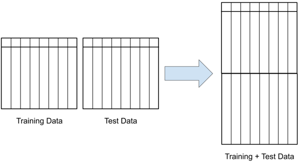
它的工作原理通过图 4 和下面的代码就能轻松理解。
import pandas as pd
from sklearn import preprocessing
# read training data
train = pd.read_csv("../input/cat_train.csv")
#read test data
test = pd.read_csv("../input/cat_test.csv")
# create a fake target column for test data
# since this column doesn't exist
test.loc[:, "target"] = -1
# concatenate both training and test data
data = pd.concat([train, test]).reset_index(drop=True)
# make a list of features we are interested in
# id and target is something we should not encode
features = [x for x in train.columns if x not in ["id", "target"]]
# loop over the features list
for feat in features:
    # create a new instance of LabelEncoder for each feature
    lbl_enc = preprocessing.LabelEncoder()
    # note the trick here
    # since its categorical data, we fillna with a string
    # and we convert all the data to string type
    # so, no matter its int or float, its converted to string
    # int/float but categorical!!!
    temp_col = data[feat].fillna("NONE").astype(str).values
    # we can use fit_transform here as we do not
    # have any extra test data that we need to
    # transform on separately
    data.loc[:, feat] = lbl_enc.fit_transform(temp_col)
# split the training and test data again
train = data[data.target != -1].reset_index(drop=True)
test = data[data.target == -1].reset_index(drop=True)
这个技巧适用于你已经拥有测试数据集的问题。必须注意,这个技巧在线上环境中是行不通的。例如,假设你在一个构建实时竞价(real-time bidding,RTB)解决方案的公司工作。RTB 系统会针对他们在网上看到的每一个用户出价,以购买广告位。用于这种模型的特征可能包括用户在网站上浏览过的页面。假设特征就是用户最后访问的五个类别/页面。在这种情况下,如果网站引入新的类别,我们将无法再准确预测。我们的模型在这种情况下会失败。这种情况可以通过使用「未知(unknown)」类别来避免。
在我们的 cat-in-the-dat 数据集中,ord_2 列里已经有了未知值。
In [X]: df.ord_2.fillna("NONE").value_counts()
Out[X]: Freezing       142726
Warm           124239
Cold            97822
Boiling Hot     84790
Hot             67508
Lava Hot        64840
NONE            18075
Name: ord_2, dtype: int64
我们可以把「NONE」当作未知。这样,如果在线上测试期间出现我们从未见过的新类别,就把它们标记为「NONE」。
这与自然语言处理(natural language processing,NLP)问题非常相似。我们总是基于一个固定的词表(vocabulary)来构建模型。词表越大,模型就越大。像 BERT 这样的 Transformer 模型是在大约 30000 个单词(针对英语)上训练的。所以,当出现一个新词时,我们会把它标记为 UNK(unknown,未知)。
所以,你要么假设测试数据会有与训练数据相同的类别,要么在训练中引入一个稀有或未知类别,以应对测试数据中的新类别。
让我们看看填充 NaN 值后 ord_4 列的值计数:
In [X]: df.ord_4.fillna("NONE").value_counts()
Out[X]: N       39978
P       37890
Y       36657
A       36633
R       33045
U       32897
. . .
K       21676
I       19805
NONE    17930
D       17284
F       16721
W        8268
Z        5790
S        4595
G        3404
V        3107
J        1950
L        1657
Name: ord_4, dtype: int64
我们看到有些值只出现几千次,有些则出现近 40000 次。NaN 也出现很多。请注意,我从输出中删除了一些值。
我们现在可以定义把一个值称为「稀有」的标准。假设这一列中一个值被认为是稀有值的条件是计数小于 2000。这样看来,J 和 L 可以被标记为稀有值。用 pandas 根据计数阈值替换类别非常容易。让我们看看怎么做。
In [X]: df.ord_4 = df.ord_4.fillna("NONE")
In [X]: df.loc[
...:     df["ord_4"].value_counts()[df["ord_4"]].values < 2000,
...:     "ord_4"
...: ] = "RARE"
In [X]: df.ord_4.value_counts()
Out[X]: N       39978
P       37890
Y       36657
A       36633
R       33045
U       32897
M       32504
.
.
.
B       25212
E       21871
K       21676
I       19805
NONE    17930
D       17284
F       16721
W        8268
Z        5790
S        4595
RARE     3607
G        3404
V        3107
Name: ord_4, dtype: int64
我们说,只要某个类别的值计数小于 2000,就把它替换为 rare。所以,现在对于测试数据,所有新的、未见过的类别都会被映射到「RARE」,所有缺失值都会被映射到「NONE」。
这种方法还能确保模型在线上环境中也能正常工作,即使出现了新类别。
现在,我们有了处理任何包含类别变量的问题所需的一切。让我们尝试构建第一个模型,并逐步改进它的性能。
在进行任何模型构建之前,处理好交叉验证是必不可少的。我们已经看到了标签/目标分布,并且知道这是一个目标有偏的二分类问题。因此,这里我们将使用分层 K 折(StratifiedKFold)来划分数据。
# create_folds.py
# import pandas and model_selection module of scikit-learn
import pandas as pd
from sklearn import model_selection

if __name__ == "__main__":
    # Read training data
    df = pd.read_csv("../input/cat_train.csv")
    # we create a new column called kfold and fill it with -1
    df["kfold"] = -1
    # the next step is to randomize the rows of the data
    df = df.sample(frac=1).reset_index(drop=True)
    # fetch labels
    y = df.target.values
    # initiate the kfold class from model_selection module
    kf = model_selection.StratifiedKFold(n_splits=5)
    # fill the new kfold column
    for f, (t_, v_) in enumerate(kf.split(X=df, y=y)):
        df.loc[v_, 'kfold'] = f
    # save the new csv with kfold column
    df.to_csv("../input/cat_train_folds.csv", index=False)
我们现在可以检查新的折 csv,看看每一折的样本数:
In [X]: import pandas as pd
In [X]: df = pd.read_csv("../input/cat_train_folds.csv")
In [X]: df.kfold.value_counts()
Out[X]: 4    120000
3    120000
2    120000
1    120000
0    120000
Name: kfold, dtype: int64
所有折都有 120000 个样本。这是符合预期的,因为训练数据有 600000 个样本,而我们做了五折。到目前为止,一切顺利。
现在,我们还可以检查每一折的目标分布。
In [X]: df[df.kfold==0].target.value_counts()
Out[X]: 0    97536
1    22464
Name: target, dtype: int64

In [X]: df[df.kfold==1].target.value_counts()
Out[X]: 0    97536
1    22464
Name: target, dtype: int64

In [X]: df[df.kfold==2].target.value_counts()
Out[X]: 0    97535
1    22465
Name: target, dtype: int64

In [X]: df[df.kfold==3].target.value_counts()
Out[X]: 0    97535
1    22465
Name: target, dtype: int64

In [X]: df[df.kfold==4].target.value_counts()
Out[X]: 0    97535
1    22465
Name: target, dtype: int64
我们看到每一折中目标的分布都相同。这正是我们需要的。它也可以是相似的,并不一定要每次都完全相同。现在,当我们构建模型时,每一折的目标分布都会相同。
我们能构建的最简单的模型之一,就是对所有数据做独热编码,然后使用逻辑回归(logistic regression)。
# ohe_logres.py
import pandas as pd
from sklearn import linear_model
from sklearn import metrics
from sklearn import preprocessing

def run(fold):
    # load the full training data with folds
    df = pd.read_csv("../input/cat_train_folds.csv")
    # all columns are features except id, target and kfold columns
    features = [
        f for f in df.columns if f not in ("id", "target", "kfold")
    ]
    # fill all NaN values with NONE
    # note that I am converting all columns to "strings"
    # it doesn't matter because all are categories
    for col in features:
        df.loc[:, col] = df[col].astype(str).fillna("NONE")
    # get training data using folds
    df_train = df[df.kfold != fold].reset_index(drop=True)
    # get validation data using folds
    df_valid = df[df.kfold == fold].reset_index(drop=True)
    # initialize OneHotEncoder from scikit-learn
    ohe = preprocessing.OneHotEncoder()
    # fit ohe on training + validation features
    full_data = pd.concat(
        [df_train[features], df_valid[features]], axis=0
    )
    ohe.fit(full_data[features])
    # transform training data
    x_train = ohe.transform(df_train[features])
    # transform validation data
    x_valid = ohe.transform(df_valid[features])
    # initialize Logistic Regression model
    model = linear_model.LogisticRegression()
    # fit model on training data (ohe)
    model.fit(x_train, df_train.target.values)
    # predict on validation data
    # we need the probability values as we are calculating AUC
    # we will use the probability of 1s
    valid_preds = model.predict_proba(x_valid)[:, 1]
    # get roc auc score
    auc = metrics.roc_auc_score(df_valid.target.values, valid_preds)
    # print auc
    print(auc)

if __name__ == "__main__":
    # run function for fold = 0
    # we can just replace this number and
    # run this for any fold
    run(0)
那么,这里发生了什么?
我们创建了一个函数:给定折号,把数据划分为训练集和验证集,处理 NaN 值,对所有数据应用独热编码,并训练一个简单的逻辑回归模型。
当我们运行这段代码时,它会产生如下输出:
❯ python ohe_logres.py
/home/abhishek/miniconda3/envs/ml/lib/python3.7/sitepackages/sklearn/linear_model/_logistic.py:939: ConvergenceWarning: lbfgs failed to converge (status=1): STOP: TOTAL NO. of ITERATIONS REACHED LIMIT. Increase the number of iterations (max_iter) or scale the data as shown in: https://scikit-learn.org/stable/modules/preprocessing.html. Please also refer to the documentation for alternative solver options: https://scikit-learn.org/stable/modules/linear_model.html#logisticregression extra_warning_msg=_LOGISTIC_SOLVER_CONVERGENCE_MSG)
0.7847865042255127
有一些警告。看起来逻辑回归在最大迭代次数内没有收敛。我们没有调整参数,所以这没关系。我们看到 AUC 约为 0.785。
现在,让我们对代码做一点小改动,在所有折上运行它。
# ohe_logres.py
. . .
# initialize Logistic Regression model
model = linear_model.LogisticRegression()
# fit model on training data (ohe)
model.fit(x_train, df_train.target.values)
# predict on validation data
# we need the probability values as we are calculating AUC
# we will use the probability of 1s
valid_preds = model.predict_proba(x_valid)[:, 1]
# get roc auc score
auc = metrics.roc_auc_score(df_valid.target.values, valid_preds)
# print auc
print(f"Fold = {fold}, AUC = {auc}")

if __name__ == "__main__":
    for fold_ in range(5):
        run(fold_)
请注意,我们没有做太多改动,所以我只展示了代码中的一些行,其中部分行有变化。
这给出:
❯ python -W ignore ohe_logres.py
Fold = 0, AUC = 0.7847865042255127
Fold = 1, AUC = 0.7853553605899214
Fold = 2, AUC = 0.7879321942914885
Fold = 3, AUC = 0.7870315929550808
Fold = 4, AUC = 0.7864668243125608
注意,我使用「-W ignore」来忽略所有警告。
我们看到各折的 AUC 分数相当稳定。平均 AUC 是 0.78631449527。对我们的第一个模型来说相当不错!
很多人会用基于树的模型(比如随机森林)来开始解决这类问题。在这个数据集上应用随机森林时,我们可以不用独热编码,而是像之前讨论的那样使用标签编码,把每一列的每个特征都转换为整数。
代码与独热编码的代码差别不大。让我们来看一下。
# lbl_rf.py
import pandas as pd
from sklearn import ensemble
from sklearn import metrics
from sklearn import preprocessing

def run(fold):
    # load the full training data with folds
    df = pd.read_csv("../input/cat_train_folds.csv")
    # all columns are features except id, target and kfold columns
    features = [
        f for f in df.columns if f not in ("id", "target", "kfold")
    ]
    # fill all NaN values with NONE
    # note that I am converting all columns to "strings"
    # it doesnt matter because all are categories
    for col in features:
        df.loc[:, col] = df[col].astype(str).fillna("NONE")
    # now its time to label encode the features
    for col in features:
        # initialize LabelEncoder for each feature column
        lbl = preprocessing.LabelEncoder()
        # fit label encoder on all data
        lbl.fit(df[col])
        # transform all the data
        df.loc[:, col] = lbl.transform(df[col])
    # get training data using folds
    df_train = df[df.kfold != fold].reset_index(drop=True)
    # get validation data using folds
    df_valid = df[df.kfold == fold].reset_index(drop=True)
    # get training data
    x_train = df_train[features].values
    # get validation data
    x_valid = df_valid[features].values
    # initialize random forest model
    model = ensemble.RandomForestClassifier(n_jobs=-1)
    # fit model on training data (ohe)
    model.fit(x_train, df_train.target.values)
    # predict on validation data
    # we need the probability values as we are calculating AUC
    # we will use the probability of 1s
    valid_preds = model.predict_proba(x_valid)[:, 1]
    # get roc auc score
    auc = metrics.roc_auc_score(df_valid.target.values, valid_preds)
    # print auc
    print(f"Fold = {fold}, AUC = {auc}")

if __name__ == "__main__":
    for fold_ in range(5):
        run(fold_)
我们使用 scikit-learn 的随机森林,并去掉了独热编码。我们使用标签编码来代替独热编码。分数如下:
❯ python lbl_rf.py
Fold = 0, AUC = 0.7167390828113697
Fold = 1, AUC = 0.7165459672958506
Fold = 2, AUC = 0.7159709909587376
Fold = 3, AUC = 0.7161589664189556
Fold = 4, AUC = 0.7156020216155978
哇!差别巨大!没有做任何超参数调优的随机森林模型,表现比简单的逻辑回归差得多。
这也是我们应该总是先从简单模型入手的原因。随机森林的粉丝会从这里开始,并忽略逻辑回归模型,认为它是一个太简单的模型,不可能带来比随机森林更好的价值。这种人会犯一个大错误。在我们的随机森林实现中,各折完成的时间比逻辑回归长得多。所以,我们不仅 AUC 更差,完成训练的时间也长得多。请注意,随机森林的推理(inference)也很耗时,而且占用的空间也大得多。
如果我们愿意,也可以尝试在稀疏的独热编码数据上运行随机森林,但那会花费大量时间。我们还可以尝试用奇异值分解(singular value decomposition)来降维稀疏的独热编码矩阵。这是自然语言处理中提取主题的一种非常常见的方法。
# ohe_svd_rf.py
import pandas as pd
from scipy import sparse
from sklearn import decomposition
from sklearn import ensemble
from sklearn import metrics
from sklearn import preprocessing

def run(fold):
    # load the full training data with folds
    df = pd.read_csv("../input/cat_train_folds.csv")
    # all columns are features except id, target and kfold columns
    features = [
        f for f in df.columns if f not in ("id", "target", "kfold")
    ]
    # fill all NaN values with NONE
    # note that I am converting all columns to "strings"
    # it doesnt matter because all are categories
    for col in features:
        df.loc[:, col] = df[col].astype(str).fillna("NONE")
    # get training data using folds
    df_train = df[df.kfold != fold].reset_index(drop=True)
    # get validation data using folds
    df_valid = df[df.kfold == fold].reset_index(drop=True)
    # initialize OneHotEncoder from scikit-learn
    ohe = preprocessing.OneHotEncoder()
    # fit ohe on training + validation features
    full_data = pd.concat(
        [df_train[features], df_valid[features]], axis=0
    )
    ohe.fit(full_data[features])
    # transform training data
    x_train = ohe.transform(df_train[features])
    # transform validation data
    x_valid = ohe.transform(df_valid[features])
    # initialize Truncated SVD
    # we are reducing the data to 120 components
    svd = decomposition.TruncatedSVD(n_components=120)
    # fit svd on full sparse training data
    full_sparse = sparse.vstack((x_train, x_valid))
    svd.fit(full_sparse)
    # transform sparse training data
    x_train = svd.transform(x_train)
    # transform sparse validation data
    x_valid = svd.transform(x_valid)
    # initialize random forest model
    model = ensemble.RandomForestClassifier(n_jobs=-1)
    # fit model on training data (ohe)
    model.fit(x_train, df_train.target.values)
    # predict on validation data
    # we need the probability values as we are calculating AUC
    # we will use the probability of 1s
    valid_preds = model.predict_proba(x_valid)[:, 1]
    # get roc auc score
    auc = metrics.roc_auc_score(df_valid.target.values, valid_preds)
    # print auc
    print(f"Fold = {fold}, AUC = {auc}")

if __name__ == "__main__":
    for fold_ in range(5):
        run(fold_)
我们对全部数据做独热编码,然后用训练数据 + 验证数据在稀疏矩阵上拟合 scikit-learn 的 TruncatedSVD。这样,我们把高维稀疏矩阵降到 120 个特征,然后拟合随机森林分类器。
下面是这个模型的输出:
❯ python ohe_svd_rf.py
Fold = 0, AUC = 0.7064863038754249
Fold = 1, AUC = 0.706050102937374
Fold = 2, AUC = 0.7086069243167242
Fold = 3, AUC = 0.7066819080085971
Fold = 4, AUC = 0.7058154015055585
我们看到它甚至更差了。看起来这个问题的最佳方法是独热编码加逻辑回归。随机森林似乎太耗时了。也许我们可以试试 XGBoost。如果你不了解 XGBoost,它是最流行的梯度提升(gradient boosting)算法之一。由于它是基于树的算法,我们将使用标签编码的数据。
# lbl_xgb.py
import pandas as pd
import xgboost as xgb
from sklearn import metrics
from sklearn import preprocessing

def run(fold):
    # load the full training data with folds
    df = pd.read_csv("../input/cat_train_folds.csv")
    # all columns are features except id, target and kfold columns
    features = [
        f for f in df.columns if f not in ("id", "target", "kfold")
    ]
    # fill all NaN values with NONE
    # note that I am converting all columns to "strings"
    # it doesnt matter because all are categories
    for col in features:
        df.loc[:, col] = df[col].astype(str).fillna("NONE")
    # now it's time to label encode the features
    for col in features:
        # initialize LabelEncoder for each feature column
        lbl = preprocessing.LabelEncoder()
        # fit label encoder on all data
        lbl.fit(df[col])
        # transform all the data
        df.loc[:, col] = lbl.transform(df[col])
    # get training data using folds
    df_train = df[df.kfold != fold].reset_index(drop=True)
    # get validation data using folds
    df_valid = df[df.kfold == fold].reset_index(drop=True)
    # get training data
    x_train = df_train[features].values
    # get validation data
    x_valid = df_valid[features].values
    # initialize xgboost model
    model = xgb.XGBClassifier(
        n_jobs=-1, max_depth=7, n_estimators=200
    )
    # fit model on training data (ohe)
    model.fit(x_train, df_train.target.values)
    # predict on validation data
    # we need the probability values as we are calculating AUC
    # we will use the probability of 1s
    valid_preds = model.predict_proba(x_valid)[:, 1]
    # get roc auc score
    auc = metrics.roc_auc_score(df_valid.target.values, valid_preds)
    # print auc
    print(f"Fold = {fold}, AUC = {auc}")

if __name__ == "__main__":
    for fold_ in range(5):
        run(fold_)
必须指出,在这段代码中,我稍微修改了 xgboost 的参数。xgboost 默认的 max_depth 是 3,我把它改成了 7,还把估计器数量(n_estimators)从 100 改成了 200。
这个模型的五折分数如下:
❯ python lbl_xgb.py
Fold = 0, AUC = 0.7656768851999011
Fold = 1, AUC = 0.7633006564148015
Fold = 2, AUC = 0.7654277821434345
Fold = 3, AUC = 0.7663609758878182
Fold = 4, AUC = 0.764914671468069
我们看到分数比未做任何调优的普通随机森林好得多,而且通过更多的超参数调优,我们可能还能进一步提高。
你也可以尝试一些特征工程,比如删除一些对模型没有任何价值的列,等等。但看起来在这里我们做不了太多来展示模型的改进。让我们换一个包含大量类别变量的数据集。另一个著名的数据集是美国成人普查数据(US adult census data)。这个数据集包含一些特征,你的任务是预测收入档位。让我们看看这个数据集。图 5 显示了该数据集中的一些列。
图 5:成人数据集(adult dataset)中若干列的截图⁶
| age | education | marital.status | race | sex | capital.loss | income | |
|---|---|---|---|---|---|---|---|
| 0 | 06 | HS-grad | Widowed | White | Female | 4356 | <=50K |
| 1 | 82 | HS-grad | Widowed | White | Female | 4356 | <=50K |
| 2 | 66 | Some-college | Widowed | Black | Female | 4356 | <=50K |
| 3 | 54 | 7th-8th | Divorced | White | Female | 3900 | <=50K |
| 4 | 41 | Some-college | Separated | White | Female | 3900 | <=50K |
| … | … | … | … | … | … | ||
| 32556 | 22 | Some-college | Never-married | White | Male | 0 | <=50K |
| 32557 | 27 | Assoc-acdm | Married-civ-spouse | White | Female | 0 | <=50K |
| 32558 | 40 | HS-grad | Married-civ-spouse | White | Male | 0 | >50K |
| 32559 | 58 | HS-grad | Widowed | White | Female | 0 | <=50K |
| 32560 | 22 | HS-grad | Never-married | White | Male | 0 | <=50K |
该数据集包含以下列:
- age
- workclass
- fnlwgt
- education
- education.num
- marital.status
- occupation
- relationship
- race
- sex
- capital.gain
- capital.loss
- hours.per.week
6 https://archive.ics.uci.edu/ml/datasets/adult
- native.country
- income
这些列大多不言自明。那些不清楚的,我们可以不管它。让我们先试着构建一个模型。
我们看到 income 列是字符串。让我们对这一列做一下值计数。
In [X]: import pandas as pd
In [X]: df = pd.read_csv("../input/adult.csv")
In [X]: df.income.value_counts()
Out[X]: <=50K    24720
>50K      7841
我们看到有 7841 个实例的收入高于 50000 美元。这大约占样本总数的 24%。因此,我们将保持与 cat-in-the-dat 数据集相同的评估指标,即 AUC。在开始建模之前,为了简单起见,我们将删除几个数值列,即:
- fnlwgt
- age
- capital.gain
- capital.loss
- hours.per.week
让我们快速用独热编码加逻辑回归试试,看看会发生什么。第一步永远是做交叉验证。这里我就不展示这部分代码了。留作读者的练习。
# ohe_logres.py
import pandas as pd
from sklearn import linear_model
from sklearn import metrics
from sklearn import preprocessing

def run(fold):
    # load the full training data with folds
    df = pd.read_csv("../input/adult_folds.csv")
    # list of numerical columns
    num_cols = [
        "fnlwgt",
        "age",
        "capital.gain",
        "capital.loss",
        "hours.per.week"
    ]
    # drop numerical columns
    df = df.drop(num_cols, axis=1)
    # map targets to 0s and 1s
    target_mapping = {
        "<=50K": 0,
        ">50K": 1
    }
    df.loc[:, "income"] = df.income.map(target_mapping)
    # all columns are features except income and kfold columns
    features = [
        f for f in df.columns if f not in ("kfold", "income")
    ]
    # fill all NaN values with NONE
    # note that I am converting all columns to "strings"
    # it doesnt matter because all are categories
    for col in features:
        df.loc[:, col] = df[col].astype(str).fillna("NONE")
    # get training data using folds
    df_train = df[df.kfold != fold].reset_index(drop=True)
    # get validation data using folds
    df_valid = df[df.kfold == fold].reset_index(drop=True)
    # initialize OneHotEncoder from scikit-learn
    ohe = preprocessing.OneHotEncoder()
    # fit ohe on training + validation features
    full_data = pd.concat(
        [df_train[features], df_valid[features]], axis=0
    )
    ohe.fit(full_data[features])
    # transform training data
    x_train = ohe.transform(df_train[features])
    # transform validation data
    x_valid = ohe.transform(df_valid[features])
    # initialize Logistic Regression model
    model = linear_model.LogisticRegression()
    # fit model on training data (ohe)
    model.fit(x_train, df_train.income.values)
    # predict on validation data
    # we need the probability values as we are calculating AUC
    # we will use the probability of 1s
    valid_preds = model.predict_proba(x_valid)[:, 1]
    # get roc auc score
    auc = metrics.roc_auc_score(df_valid.income.values, valid_preds)
    # print auc
    print(f"Fold = {fold}, AUC = {auc}")

if __name__ == "__main__":
    for fold_ in range(5):
        run(fold_)
当我们运行这段代码时,会得到:
❯ python -W ignore ohe_logres.py
Fold = 0, AUC = 0.8794809708119079
Fold = 1, AUC = 0.8875785068274882
Fold = 2, AUC = 0.8852609687685753
Fold = 3, AUC = 0.8681236223251438
Fold = 4, AUC = 0.8728581541840037
对一个如此简单的模型来说,这是一个非常好的 AUC!
现在,让我们试试不做任何超参数调优的标签编码 xgboost。
# lbl_xgb.py
import pandas as pd
import xgboost as xgb
from sklearn import metrics
from sklearn import preprocessing

def run(fold):
    # load the full training data with folds
    df = pd.read_csv("../input/adult_folds.csv")
    # list of numerical columns
    num_cols = [
        "fnlwgt",
        "age",
        "capital.gain",
        "capital.loss",
        "hours.per.week"
    ]
    # drop numerical columns
    df = df.drop(num_cols, axis=1)
    # map targets to 0s and 1s
    target_mapping = {
        "<=50K": 0,
        ">50K": 1
    }
    df.loc[:, "income"] = df.income.map(target_mapping)
    # all columns are features except kfold & income columns
    features = [
        f for f in df.columns if f not in ("kfold", "income")
    ]
    # fill all NaN values with NONE
    # note that I am converting all columns to "strings"
    # it doesnt matter because all are categories
    for col in features:
        df.loc[:, col] = df[col].astype(str).fillna("NONE")
    # now its time to label encode the features
    for col in features:
        # initialize LabelEncoder for each feature column
        lbl = preprocessing.LabelEncoder()
        # fit label encoder on all data
        lbl.fit(df[col])
        # transform all the data
        df.loc[:, col] = lbl.transform(df[col])
    # get training data using folds
    df_train = df[df.kfold != fold].reset_index(drop=True)
    # get validation data using folds
    df_valid = df[df.kfold == fold].reset_index(drop=True)
    # get training data
    x_train = df_train[features].values
    # get validation data
    x_valid = df_valid[features].values
    # initialize xgboost model
    model = xgb.XGBClassifier(
        n_jobs=-1
    )
    # fit model on training data (ohe)
    model.fit(x_train, df_train.income.values)
    # predict on validation data
    # we need the probability values as we are calculating AUC
    # we will use the probability of 1s
    valid_preds = model.predict_proba(x_valid)[:, 1]
    # get roc auc score
    auc = metrics.roc_auc_score(df_valid.income.values, valid_preds)
    # print auc
    print(f"Fold = {fold}, AUC = {auc}")

if __name__ == "__main__":
    for fold_ in range(5):
        run(fold_)
让我们运行它!
❯ python lbl_xgb.py
Fold = 0, AUC = 0.8800810634234078
Fold = 1, AUC = 0.886811884948154
Fold = 2, AUC = 0.8854421433318472
Fold = 3, AUC = 0.8676319549361007
Fold = 4, AUC = 0.8714450054900602
这看起来已经很不错了。让我们看看把 max_depth 提高到 7、n_estimators 提高到 200 时的分数。
❯ python lbl_xgb.py
Fold = 0, AUC = 0.8764108944332032
Fold = 1, AUC = 0.8840708537662638
Fold = 2, AUC = 0.8816601162613102
Fold = 3, AUC = 0.8662335762581732
Fold = 4, AUC = 0.8698983461709926
看起来并没有改善。
这说明一个数据集的参数并不能迁移到另一个数据集。我们必须再次尝试调参,不过我们会在接下来的章节中更详细地做这件事。
现在,让我们尝试在不调参的情况下,把数值特征纳入 xgboost 模型。
# lbl_xgb_num.py
import pandas as pd
import xgboost as xgb
from sklearn import metrics
from sklearn import preprocessing

def run(fold):
    # load the full training data with folds
    df = pd.read_csv("../input/adult_folds.csv")
    # list of numerical columns
    num_cols = [
        "fnlwgt",
        "age",
        "capital.gain",
        "capital.loss",
        "hours.per.week"
    ]
    # map targets to 0s and 1s
    target_mapping = {
        "<=50K": 0,
        ">50K": 1
    }
    df.loc[:, "income"] = df.income.map(target_mapping)
    # all columns are features except kfold & income columns
    features = [
        f for f in df.columns if f not in ("kfold", "income")
    ]
    # fill all NaN values with NONE
    # note that I am converting all columns to "strings"
    # it doesnt matter because all are categories
    for col in features:
        # do not encode the numerical columns
        if col not in num_cols:
            df.loc[:, col] = df[col].astype(str).fillna("NONE")
    # now its time to label encode the features
    for col in features:
        if col not in num_cols:
            # initialize LabelEncoder for each feature column
            lbl = preprocessing.LabelEncoder()
            # fit label encoder on all data
            lbl.fit(df[col])
            # transform all the data
            df.loc[:, col] = lbl.transform(df[col])
    # get training data using folds
    df_train = df[df.kfold != fold].reset_index(drop=True)
    # get validation data using folds
    df_valid = df[df.kfold == fold].reset_index(drop=True)
    # get training data
    x_train = df_train[features].values
    # get validation data
    x_valid = df_valid[features].values
    # initialize xgboost model
    model = xgb.XGBClassifier(
        n_jobs=-1
    )
    # fit model on training data (ohe)
    model.fit(x_train, df_train.income.values)
    # predict on validation data
    # we need the probability values as we are calculating AUC
    # we will use the probability of 1s
    valid_preds = model.predict_proba(x_valid)[:, 1]
    # get roc auc score
    auc = metrics.roc_auc_score(df_valid.income.values, valid_preds)
    # print auc
    print(f"Fold = {fold}, AUC = {auc}")

if __name__ == "__main__":
    for fold_ in range(5):
        run(fold_)
所以,我们保留数值列,只是不对它们做标签编码。这样,我们的最终特征矩阵就由数值列(原样)和编码后的类别列组成。任何基于树的算法都能轻松处理这种混合。
请注意,使用基于树的模型时我们不需要归一化数据。然而,在使用线性模型(如逻辑回归)时,这是必须做且不能遗漏的关键一步。
现在让我们运行这个脚本!
❯ python lbl_xgb_num.py
Fold = 0, AUC = 0.9209790185449889
Fold = 1, AUC = 0.9247157449144706
Fold = 2, AUC = 0.9269329887598243
Fold = 3, AUC = 0.9119349082169275
Fold = 4, AUC = 0.9166408030141667
哇哦!
这是一个非常棒的分数!
现在,我们可以尝试添加一些特征。我们将取所有的类别列,创建所有二阶组合。请看下面代码片段中的 feature_engineering 函数,了解具体做法。
# lbl_xgb_num_feat.py
import itertools
import pandas as pd
import xgboost as xgb
from sklearn import metrics
from sklearn import preprocessing

def feature_engineering(df, cat_cols):
    """
    This function is used for feature engineering

    :param df: the pandas dataframe with train/test data
    :param cat_cols: list of categorical columns
    :return: dataframe with new features
    """
    # this will create all 2-combinations of values
    # in this list
    # for example:
    # list(itertools.combinations([1,2,3], 2)) will return
    # [(1, 2), (1, 3), (2, 3)]
    combi = list(itertools.combinations(cat_cols, 2))
    for c1, c2 in combi:
        df.loc[ :, c1 + "_" + c2 ] = df[c1].astype(str) + "_" + df[c2].astype(str)
    return df

def run(fold):
    # load the full training data with folds
    df = pd.read_csv("../input/adult_folds.csv")
    # list of numerical columns
    num_cols = [
        "fnlwgt",
        "age",
        "capital.gain",
        "capital.loss",
        "hours.per.week"
    ]
    # map targets to 0s and 1s
    target_mapping = {
        "<=50K": 0,
        ">50K": 1
    }
    df.loc[:, "income"] = df.income.map(target_mapping)
    # list of categorical columns for feature engineering
    cat_cols = [
        c for c in df.columns if c not in num_cols and c not in ("kfold", "income")
    ]
    # add new features
    df = feature_engineering(df, cat_cols)
    # all columns are features except kfold & income columns
    features = [
        f for f in df.columns if f not in ("kfold", "income")
    ]
    # fill all NaN values with NONE
    # note that I am converting all columns to "strings"
    # it doesnt matter because all are categories
    for col in features:
        # do not encode the numerical columns
        if col not in num_cols:
            df.loc[:, col] = df[col].astype(str).fillna("NONE")
    # now its time to label encode the features
    for col in features:
        if col not in num_cols:
            # initialize LabelEncoder for each feature column
            lbl = preprocessing.LabelEncoder()
            # fit label encoder on all data
            lbl.fit(df[col])
            # transform all the data
            df.loc[:, col] = lbl.transform(df[col])
    # get training data using folds
    df_train = df[df.kfold != fold].reset_index(drop=True)
    # get validation data using folds
    df_valid = df[df.kfold == fold].reset_index(drop=True)
    # get training data
    x_train = df_train[features].values
    # get validation data
    x_valid = df_valid[features].values
    # initialize xgboost model
    model = xgb.XGBClassifier(
        n_jobs=-1
    )
    # fit model on training data (ohe)
    model.fit(x_train, df_train.income.values)
    # predict on validation data
    # we need the probability values as we are calculating AUC
    # we will use the probability of 1s
    valid_preds = model.predict_proba(x_valid)[:, 1]
    # get roc auc score
    auc = metrics.roc_auc_score(df_valid.income.values, valid_preds)
    # print auc
    print(f"Fold = {fold}, AUC = {auc}")

if __name__ == "__main__":
    for fold_ in range(5):
        run(fold_)
这是一种非常朴素的从类别列创建特征的方法。你应该先看看数据,弄清楚哪些组合最有意义。如果使用这种方法,你可能会创建出大量特征,在这种情况下,你需要使用某种特征选择(feature selection)来选出最好的特征。我们稍后会了解更多关于特征选择的内容。现在让我们看看分数。
❯ python lbl_xgb_num_feat.py
Fold = 0, AUC = 0.9211483465031423
Fold = 1, AUC = 0.9251499446866125
Fold = 2, AUC = 0.9262344766486692
Fold = 3, AUC = 0.9114264068794995
Fold = 4, AUC = 0.9177914453099201
看起来即使不修改任何超参数,仅仅添加一堆特征,我们也能稍微提高各折的分数。让我们看看把 max_depth 提高到 7 是否有帮助。
❯ python lbl_xgb_num_feat.py
Fold = 0, AUC = 0.9286668430204137
Fold = 1, AUC = 0.9329340656165378
Fold = 2, AUC = 0.9319817543218744
Fold = 3, AUC = 0.919046187194538
Fold = 4, AUC = 0.9245692057162671
再一次,我们成功改进了模型。
请注意,我们还没有使用稀有值、二元特征、独热编码与标签编码特征的组合以及其他几种方法。
从类别特征中进行特征工程的另一种方法是使用目标编码(target encoding)。不过,在这里你必须非常小心,因为这可能会让模型过拟合。目标编码是一种把给定特征中的每个类别映射到其目标均值(mean target value)的技术,但这样做必须始终以交叉验证的方式进行。这意味着你要做的第一件事是创建折,然后用这些折为数据的不同列创建目标编码特征,就像你在折上拟合并预测模型一样。所以,如果你创建了 5 折,就必须创建 5 次目标编码,这样最终每一折中变量的编码都不是由同一折推导出来的。然后当你拟合模型时,必须再次使用相同的折。对未见过的测试数据的目标编码,可以从完整的训练数据中推导,也可以是全部 5 折的平均值。
让我们看看如何在同一个成人数据集上使用目标编码,以便进行比较。
# target_encoding.py
import copy
import pandas as pd
from sklearn import metrics
from sklearn import preprocessing
import xgboost as xgb

def mean_target_encoding(data):
    # make a copy of dataframe
    df = copy.deepcopy(data)
    # list of numerical columns
    num_cols = [
        "fnlwgt",
        "age",
        "capital.gain",
        "capital.loss",
        "hours.per.week"
    ]
    # map targets to 0s and 1s
    target_mapping = {
        "<=50K": 0,
        ">50K": 1
    }
    df.loc[:, "income"] = df.income.map(target_mapping)
    # all columns are features except income and kfold columns
    features = [
        f for f in df.columns if f not in ("kfold", "income") and f not in num_cols
    ]
    # fill all NaN values with NONE
    # note that I am converting all columns to "strings"
    # it doesnt matter because all are categories
    for col in features:
        # do not encode the numerical columns
        if col not in num_cols:
            df.loc[:, col] = df[col].astype(str).fillna("NONE")
    # now its time to label encode the features
    for col in features:
        if col not in num_cols:
            # initialize LabelEncoder for each feature column
            lbl = preprocessing.LabelEncoder()
            # fit label encoder on all data
            lbl.fit(df[col])
            # transform all the data
            df.loc[:, col] = lbl.transform(df[col])
    # a list to store 5 validation dataframes
    encoded_dfs = []
    # go over all folds
    for fold in range(5):
        # fetch training and validation data
        df_train = df[df.kfold != fold].reset_index(drop=True)
        df_valid = df[df.kfold == fold].reset_index(drop=True)
        # for all feature columns, i.e. categorical columns
        for column in features:
            # create dict of category:mean target
            mapping_dict = dict(
                df_train.groupby(column)["income"].mean()
            )
            # column_enc is the new column we have with mean encoding
            df_valid.loc[
                :,
                column + "_enc"
            ] = df_valid[column].map(mapping_dict)
        # append to our list of encoded validation dataframes
        encoded_dfs.append(df_valid)
    # create full data frame again and return
    encoded_df = pd.concat(encoded_dfs, axis=0)
    return encoded_df

def run(df, fold):
    # note that folds are same as before
    # get training data using folds
    df_train = df[df.kfold != fold].reset_index(drop=True)
    # get validation data using folds
    df_valid = df[df.kfold == fold].reset_index(drop=True)
    # all columns are features except income and kfold columns
    features = [
        f for f in df.columns if f not in ("kfold", "income")
    ]
    # scale training data
    x_train = df_train[features].values
    # scale validation data
    x_valid = df_valid[features].values
    # initialize xgboost model
    model = xgb.XGBClassifier(
        n_jobs=-1,
        max_depth=7
    )
    # fit model on training data (ohe)
    model.fit(x_train, df_train.income.values)
    # predict on validation data
    # we need the probability values as we are calculating AUC
    # we will use the probability of 1s
    valid_preds = model.predict_proba(x_valid)[:, 1]
    # get roc auc score
    auc = metrics.roc_auc_score(df_valid.income.values, valid_preds)
    # print auc
    print(f"Fold = {fold}, AUC = {auc}")

if __name__ == "__main__":
    # read data
    df = pd.read_csv("../input/adult_folds.csv")
    # create mean target encoded categories and
    # munge data
    df = mean_target_encoding(df)
    # run training and validation for 5 folds
    for fold_ in range(5):
        run(df, fold_)
必须指出,在上面的代码片段中,做目标编码时我没有删除类别列。我保留了所有特征,并在其之上添加了目标编码特征。另外,我使用了均值。你可以使用均值、中位数、标准差或目标的任何其他函数。
让我们看看结果。
Fold = 0, AUC = 0.9332240662017529
Fold = 1, AUC = 0.9363551625140347
Fold = 2, AUC = 0.9375013544556173
Fold = 3, AUC = 0.92237621307625
Fold = 4, AUC = 0.9292131180445478
不错!看起来我们又进步了。不过,使用目标编码时你必须非常小心,因为它太容易过拟合了。使用目标编码时,最好在编码值上做一些平滑(smoothing)或添加噪声。scikit-learn 有一个 contrib 仓库,里面带有平滑的目标编码,你也可以自己实现平滑。平滑引入了某种正则化(regularization),有助于模型不过拟合。这并不难。
处理类别特征是一项复杂的任务。在各种资料中流传着大量相关信息。本章应该能帮助你开始处理任何包含类别变量的问题。不过,对于大多数问题,你只需要独热编码和标签编码就够了。要进一步改进模型,你可能还需要更多!
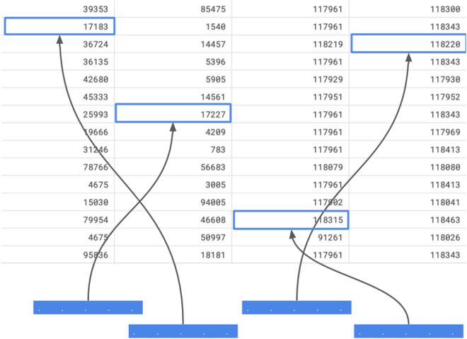
不在这份数据上跑一个神经网络,我们这一章就不能算结束。让我们来看一种叫做实体嵌入(entity embedding)的技术。在实体嵌入中,类别被表示为向量。在二值化和独热编码这两种方法中,我们也是用向量表示类别。但如果我们有数万个类别呢?这会生成巨大的矩阵,训练复杂模型会花费很长时间。因此,我们可以改用浮点值向量来表示它们。
这个想法非常简单。每个类别特征都有一个嵌入层(embedding layer)。这样,一列中的每个类别都可以映射到一个嵌入(就像自然语言处理中把单词映射到嵌入一样)。然后,你把这些嵌入重塑为扁平(flat)的向量,再拼接所有扁平化后的输入嵌入。接着加上一堆全连接层(dense layers)、一个输出层,就完成了。
图 6:类别被转换为浮点向量,即嵌入
不知为何,我觉得用 TF/Keras 来做这件事非常容易。那么,让我们看看如何用 TF/Keras 实现它。另外,这也是本书中唯一使用 TF/Keras 的例子,而且把它转换成 PyTorch 非常容易(使用 cat-in-the-dat-ii 数据集)。
# entity_emebddings.py
import os
import gc
import joblib
import pandas as pd
import numpy as np
from sklearn import metrics, preprocessing
from tensorflow.keras import layers
from tensorflow.keras import optimizers
from tensorflow.keras.models import Model, load_model
from tensorflow.keras import callbacks
from tensorflow.keras import backend as K
from tensorflow.keras import utils

def create_model(data, catcols):
    """
    This function returns a compiled tf.keras model for entity embeddings

    :param data: this is a pandas dataframe
    :param catcols: list of categorical column names
    :return: compiled tf.keras model
    """
    # init list of inputs for embeddings
    inputs = []
    # init list of outputs for embeddings
    outputs = []
    # loop over all categorical columns
    for c in catcols:
        # find the number of unique values in the column
        num_unique_values = int(data[c].nunique())
        # simple dimension of embedding calculator
        # min size is half of the number of unique values
        # max size is 50. max size depends on the number of unique
        # categories too. 50 is quite sufficient most of the times
        # but if you have millions of unique values, you might need
        # a larger dimension
        embed_dim = int(min(np.ceil((num_unique_values)/2), 50))
        # simple keras input layer with size 1
        inp = layers.Input(shape=(1,))
        # add embedding layer to raw input
        # embedding size is always 1 more than unique values in input
        out = layers.Embedding(
            num_unique_values + 1,
            embed_dim,
            name=c
        )(inp)
        # 1-d spatial dropout is the standard for emebedding layers
        # you can use it in NLP tasks too
        out = layers.SpatialDropout1D(0.3)(out)
        # reshape the input to the dimension of embedding
        # this becomes our output layer for current feature
        out = layers.Reshape(target_shape=(embed_dim, ))(out)
        # add input to input list
        inputs.append(inp)
        # add output to output list
        outputs.append(out)
    # concatenate all output layers
    x = layers.Concatenate()(outputs)
    # add a batchnorm layer.
    # from here, everything is up to you
    # you can try different architectures
    # this is the architecture I like to use
    # if you have numerical features, you should add
    # them here or in concatenate layer
    x = layers.BatchNormalization()(x)
    # a bunch of dense layers with dropout.
    # start with 1 or two layers only
    x = layers.Dense(300, activation="relu")(x)
    x = layers.Dropout(0.3)(x)
    x = layers.BatchNormalization()(x)
    x = layers.Dense(300, activation="relu")(x)
    x = layers.Dropout(0.3)(x)
    x = layers.BatchNormalization()(x)
    # using softmax and treating it as a two class problem
    # you can also use sigmoid, then you need to use only one
    # output class
    y = layers.Dense(2, activation="softmax")(x)
    # create final model
    model = Model(inputs=inputs, outputs=y)
    # compile the model
    # we use adam and binary cross entropy.
    # feel free to use something else and see how model behaves
    model.compile(loss='binary_crossentropy', optimizer='adam')
    return model

def run(fold):
    # load the full training data with folds
    df = pd.read_csv("../input/cat_train_folds.csv")
    # all columns are features except id, target and kfold columns
    features = [
        f for f in df.columns if f not in ("id", "target", "kfold")
    ]
    # fill all NaN values with NONE
    # note that I am converting all columns to "strings"
    # it doesnt matter because all are categories
    for col in features:
        df.loc[:, col] = df[col].astype(str).fillna("NONE")
    # encode all features with label encoder individually
    # in a live setting you need to save all label encoders
    for feat in features:
        lbl_enc = preprocessing.LabelEncoder()
        df.loc[:, feat] = lbl_enc.fit_transform(df[feat].values)
    # get training data using folds
    df_train = df[df.kfold != fold].reset_index(drop=True)
    # get validation data using folds
    df_valid = df[df.kfold == fold].reset_index(drop=True)
    # create tf.keras model
    model = create_model(df, features)
    # our features are lists of lists
    xtrain = [
        df_train[features].values[:, k] for k in range(len(features))
    ]
    xvalid = [
        df_valid[features].values[:, k] for k in range(len(features))
    ]
    # fetch target columns
    ytrain = df_train.target.values
    yvalid = df_valid.target.values
    # convert target columns to categories
    # this is just binarization
    ytrain_cat = utils.to_categorical(ytrain)
    yvalid_cat = utils.to_categorical(yvalid)
    # fit the model
    model.fit(
        xtrain,
        ytrain_cat,
        validation_data=(xvalid, yvalid_cat),
        verbose=1,
        batch_size=1024,
        epochs=3
    )
    # generate validation predictions
    valid_preds = model.predict(xvalid)[:, 1]
    # print roc auc score
    print(metrics.roc_auc_score(yvalid, valid_preds))
    # clear session to free up some GPU memory
    K.clear_session()

if __name__ == "__main__":
    run(0)
    run(1)
    run(2)
    run(3)
    run(4)
你会注意到,这种方法给出了最好的结果,而且如果你有 GPU,它还超级快!它还可以进一步改进,而且你不需要担心特征工程,因为神经网络会自行处理。当处理大型类别特征数据集时,这绝对值得一试。当嵌入大小与唯一类别数量相同时,就退化为独热编码了。
这一章基本上讲的都是特征工程。在下一章中,让我们看看如何对数值特征以及不同类型特征的组合做更多的特征工程。