评估指标

在处理机器学习问题时，你在现实世界中会遇到很多不同类型的指标。有时，人们甚至会创造出适合业务问题的指标。逐一介绍和解释每一种指标超出了本书的范围。相反，我们将介绍一些最常见的指标，这些指标在你刚开始做最初的几个项目时就可以使用。

在本书开头，我们介绍了监督学习（supervised learning）和无监督学习（unsupervised learning）。虽然有一些指标可以用于无监督学习，但我们只关注监督学习。原因是监督学习问题的数量远多于无监督学习，而且无监督方法的评估相当主观。

如果说到分类（classification）问题，最常用的指标有：

准确率（Accuracy）
精确率（Precision，P）
召回率（Recall，R）
F1 分数（F1 score）
ROC（受试者工作特征）曲线下面积（Area Under the ROC Curve，AUC）
对数损失（Log loss）
top-k 精确率（Precision at k，P@k）
top-k 平均精确率（Average precision at k，AP@k）
top-k 平均精确率的均值（Mean average precision at k，MAP@k）

说到回归（regression），最常用的评估指标有：

平均绝对误差（Mean Absolute Error，MAE）
均方误差（Mean Squared Error，MSE）
均方根误差（Root Mean Squared Error，RMSE）
均方根对数误差（Root Mean Squared Logarithmic Error，RMSLE）
平均百分比误差（Mean Percentage Error，MPE）
平均绝对百分比误差（Mean Absolute Percentage Error，MAPE）
R 平方（R²）

了解上述指标的工作原理并不是我们唯一需要理解的事情。我们还必须知道什么时候该用哪个指标，而这取决于你拥有什么样的数据和目标。我认为这更多取决于目标，而不是数据。

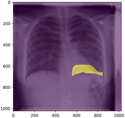
为了进一步了解这些指标，让我们从一个简单的问题开始。假设我们有一个二分类（binary classification）问题，即一个只有两个目标的问题。假设这是一个对胸部 X 光（chest x-ray）图像进行分类的问题。有些胸部 X 光图像没有问题，而有些胸部 X 光图像存在肺塌陷，也就是所谓的气胸（pneumothorax）。因此，我们的任务是构建一个分类器，给定一张胸部 X 光图像，能够检测它是否患有气胸。

Figure 1: A lung image showing pneumothorax. Image is taken from SIIM-ACR Pneumothorax Segmentation Competition 3

我们还假设气胸和非气胸的胸部 X 光图像数量相等；假设各 100 张。因此，我们有 100 个正样本（positive samples）和 100 个负样本（negative samples），总共 200 张图像。

第一步是将上述数据分成两个各含 100 张图像的相等集合，即训练集（training set）和验证集（validation set）。在这两个集合中，我们都有 50 个正样本和 50 个负样本。

3 https://www.kaggle.com/c/siim-acr-pneumothorax-segmentation

在二分类指标中，当正样本和负样本数量相等时，我们通常使用准确率、精确率、召回率和 F1。

准确率（Accuracy）

准确率（Accuracy）：它是机器学习中使用的最直接的指标之一。它定义你的模型有多准确。对于上述问题，如果你构建的模型正确分类了 90 张图像，你的准确率就是 90% 或 0.90。如果只有 83 张图像被正确分类，你的模型准确率就是 83% 或 0.83。很简单。

用 Python 计算准确率的代码也非常简单。

def accuracy(y_true, y_pred):
    """
    Function to calculate accuracy
    :param y_true: list of true values
    :param y_pred: list of predicted values
    :return: accuracy score
    """
    # initialize a simple counter for correct predictions
    correct_counter = 0
    # loop over all elements of y_true
    # and y_pred "together"
    for yt, yp in zip(y_true, y_pred):
        if yt == yp:
            # if prediction is equal to truth, increase the counter
            correct_counter += 1
    # return accuracy
    # which is correct predictions over the number of samples
    return correct_counter / len(y_true)

我们也可以使用 scikit-learn 计算准确率。

In [X]: from sklearn import metrics
...: l1 = [0,1,1,1,0,0,0,1]
...: l2 = [0,1,0,1,0,1,0,0]
...: metrics.accuracy_score(l1, l2)
Out[X]: 0.625

现在，假设我们稍微改变一下数据集，使得有 180 张胸部 X 光图像没有气胸，只有 20 张有气胸。即使在这种情况下，我们也会按照相同的正负（气胸与非气胸）目标比例创建训练集和验证集。在每个集合中，我们有 90 张非气胸图像和 10 张气胸图像。如果你说验证集中的所有图像都是非气胸，你的准确率会是多少？让我们看看；你正确分类了 90% 的图像。所以你的准确率是 90%。

但再看一次。

你甚至没有构建模型就得到了 90% 的准确率。这看起来有点没用。如果我们仔细看，会发现数据集是偏斜的（skewed），即一个类别的样本数量远超另一个类别。在这类情况下，不建议使用准确率作为评估指标，因为它不能代表数据。所以，你可能会得到很高的准确率，但在面对真实世界样本时，你的模型可能表现不佳，而且你无法向你的经理解释原因。

在这些情况下，最好看看其他指标，比如精确率（precision）。

真正例、真负例、假正例、假负例

在学习精确率之前，我们需要了解几个术语。这里我们假设有气胸的胸部 X 光图像是正类（1），没有气胸的是负类（0）。

真正例（True Positive，TP）：给定一张图像，如果你的模型预测该图像有气胸，而该图像的实际目标确实是有气胸，那么它就被认为是真正例。

真负例（True Negative，TN）：给定一张图像，如果你的模型预测该图像没有气胸，而实际目标也表明它是非气胸图像，那么它就被认为是真负例。

简单来说，如果你的模型正确预测了正类，就是真正例；如果你的模型准确预测了负类，就是真负例。

假正例（False Positive，FP）：给定一张图像，如果你的模型预测有气胸，而该图像的实际目标是非气胸，那么它就是假正例。

假负例（False Negative，FN）：给定一张图像，如果你的模型预测非气胸，而该图像的实际目标是气胸，那么它就是假负例。

简单来说，如果你的模型错误（或虚假）地预测了正类，就是假正例。如果你的模型错误（或虚假）地预测了负类，就是假负例。

让我们逐一看看这些的实现。

def true_positive(y_true, y_pred):
    """
    Function to calculate True Positives
    :param y_true: list of true values
    :param y_pred: list of predicted values
    :return: number of true positives
    """
    # initialize
    tp = 0
    for yt, yp in zip(y_true, y_pred):
        if yt == 1 and yp == 1:
            tp += 1
    return tp


def true_negative(y_true, y_pred):
    """
    Function to calculate True Negatives
    :param y_true: list of true values
    :param y_pred: list of predicted values
    :return: number of true negatives
    """
    # initialize
    tn = 0
    for yt, yp in zip(y_true, y_pred):
        if yt == 0 and yp == 0:
            tn += 1
    return tn


def false_positive(y_true, y_pred):
    """
    Function to calculate False Positives
    :param y_true: list of true values
    :param y_pred: list of predicted values
    :return: number of false positives
    """
    # initialize
    fp = 0
    for yt, yp in zip(y_true, y_pred):
        if yt == 0 and yp == 1:
            fp += 1
    return fp


def false_negative(y_true, y_pred):
    """
    Function to calculate False Negatives
    :param y_true: list of true values
    :param y_pred: list of predicted values
    :return: number of false negatives
    """
    # initialize
    fn = 0
    for yt, yp in zip(y_true, y_pred):
        if yt == 1 and yp == 0:
            fn += 1
    return fn

我在这里的实现方式非常简单，只适用于二分类。让我们来检验这些函数。

In [X]: l1 = [0,1,1,1,0,0,0,1]
...: l2 = [0,1,0,1,0,1,0,0]
In [X]: true_positive(l1, l2)
Out[X]: 2
In [X]: false_positive(l1, l2)
Out[X]: 1
In [X]: false_negative(l1, l2)
Out[X]: 2
In [X]: true_negative(l1, l2)
Out[X]: 3

如果必须用上述术语来定义准确率，我们可以这样写：

\[ \text{Accuracy} = \frac{TP + TN}{TP + TN + FP + FN} \]

现在我们可以用 Python 快速用 TP、TN、FP 和 FN 实现准确率。我们把它叫做 accuracy_v2。

def accuracy_v2(y_true, y_pred):
    """
    Function to calculate accuracy using tp/tn/fp/fn
    :param y_true: list of true values
    :param y_pred: list of predicted values
    :return: accuracy score
    """
    tp = true_positive(y_true, y_pred)
    fp = false_positive(y_true, y_pred)
    fn = false_negative(y_true, y_pred)
    tn = true_negative(y_true, y_pred)
    accuracy_score = (tp + tn) / (tp + tn + fp + fn)
    return accuracy_score

我们可以通过将其与我们之前的实现和 scikit-learn 版本进行比较来快速检查这个函数的正确性。

In [X]: l1 = [0,1,1,1,0,0,0,1]
...: l2 = [0,1,0,1,0,1,0,0]
In [X]: accuracy(l1, l2)
Out[X]: 0.625
In [X]: accuracy_v2(l1, l2)
Out[X]: 0.625
In [X]: metrics.accuracy_score(l1, l2)
Out[X]: 0.625

请注意，在这段代码中，metrics.accuracy_score 来自 scikit-learn。

太好了。所有数值都一致。这意味着我们的实现没有犯任何错误。

现在，我们可以继续讨论其他重要指标。

精确率（Precision）

第一个是精确率。精确率的定义是：

\[ \text{Precision} = \frac{TP}{TP + FP} \]

假设我们在新的偏斜数据集上构建了一个新模型，我们的模型正确识别了 90 张非气胸图像中的 80 张，以及 10 张气胸图像中的 8 张。因此，我们在 100 张图像中成功识别了 88 张。准确率因此是 0.88 或 88%。

但是，在这 100 个样本中，有 10 张非气胸图像被错误分类为有气胸，2 张气胸图像被错误分类为没有气胸。

因此，我们有：

TP：8
TN：80
FP：10
FN：2

所以，我们的精确率是 8 / (8 + 10) = 0.444。这意味着我们的模型在识别正样本（气胸）时，有 44.4% 的时间是正确的。

现在，既然我们已经实现了 TP、TN、FP 和 FN，我们就可以很容易地在 Python 中实现精确率。

def precision(y_true, y_pred):
    """
    Function to calculate precision
    :param y_true: list of true values
    :param y_pred: list of predicted values
    :return: precision score
    """
    tp = true_positive(y_true, y_pred)
    fp = false_positive(y_true, y_pred)
    precision = tp / (tp + fp)
    return precision

让我们试试这个精确率的实现。

In [X]: l1 = [0,1,1,1,0,0,0,1]
...: l2 = [0,1,0,1,0,1,0,0]
In [X]: precision(l1, l2)
Out[X]: 0.6666666666666666

看起来没问题。

召回率（Recall）

接下来是召回率。召回率的定义是：

\[ \text{Recall} = \frac{TP}{TP + FN} \]

在上述情况下，召回率是 8 / (8 + 2) = 0.80。这意味着我们的模型正确识别了 80% 的正样本。

def recall(y_true, y_pred):
    """
    Function to calculate recall
    :param y_true: list of true values
    :param y_pred: list of predicted values
    :return: recall score
    """
    tp = true_positive(y_true, y_pred)
    fn = false_negative(y_true, y_pred)
    recall = tp / (tp + fn)
    return recall

在我们这两个小列表的情况下，召回率应该是 0.5。让我们检查一下。

In [X]: l1 = [0,1,1,1,0,0,0,1]
...: l2 = [0,1,0,1,0,1,0,0]
In [X]: recall(l1, l2)
Out[X]: 0.5

这与我们计算的值一致！

对于一个『好』的模型，我们的精确率和召回率都应该是高的。我们看到在上面的例子中，召回率相当高。然而，精确率非常低！我们的模型产生了相当多的假正例，但假负例较少。在这类问题中，较少的假负例是好的，因为你不希望对实际上患有气胸的患者说他们没有气胸。那会更有害。但我们确实有很多假正例，这也不好。

大多数模型预测的是概率，当我们做预测时，通常选择 0.5 作为这个阈值（threshold）。这个阈值并不总是理想的，根据这个阈值，你的精确率和召回率的值可能会发生巨大变化。如果我们为选择的每个阈值都计算精确率和召回率，就可以在这两组值之间绘制一个图。这个图或曲线被称为精确率-召回率曲线（precision-recall curve）。

精确率-召回率曲线（Precision-Recall Curve）

在研究精确率-召回率曲线之前，让我们假设两个列表。

In [X]: y_true = [0, 0, 0, 1, 0, 0, 0, 0, 0, 0,
...:           1, 0, 0, 0, 0, 0, 0, 0, 1, 0]
In [X]: y_pred = [0.02638412, 0.11114267, 0.31620708,
...:           0.0490937,  0.0191491,  0.17554844,
...:           0.15952202, 0.03819563, 0.11639273,
...:           0.079377,   0.08584789, 0.39095342,
...:           0.27259048, 0.03447096, 0.04644807,
...:           0.03543574, 0.18521942, 0.05934905,
...:           0.61977213, 0.33056815]

所以，y_true 是我们的目标，y_pred 是一个样本被赋值为 1 的概率值。所以，现在我们看预测中的概率，而不是预测值（预测值大多数时候是以 0.5 的阈值计算的）。

precisions = []
recalls = []
# how we assumed these thresholds is a long story
thresholds = [0.0490937 , 0.05934905, 0.079377, 0.08584789, 0.11114267, 0.11639273, 0.15952202, 0.17554844, 0.18521942, 0.27259048, 0.31620708, 0.33056815, 0.39095342, 0.61977213]
# for every threshold, calculate predictions in binary
# and append calculated precisions and recalls
# to their respective lists
for i in thresholds:
    temp_prediction = [1 if x >= i else 0 for x in y_pred]
    p = precision(y_true, temp_prediction)
    r = recall(y_true, temp_prediction)
    precisions.append(p)
    recalls.append(r)

现在，我们可以绘制这些精确率和召回率的值。

plt.figure(figsize=(7, 7))
plt.plot(recalls, precisions)
plt.xlabel('Recall', fontsize=15)
plt.ylabel('Precision', fontsize=15)

图 2 显示了这样得到的精确率-召回率曲线。

Figure 2: precision-recall curve

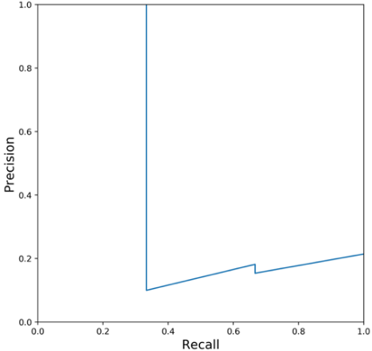
这条精确率-召回率曲线看起来和你在网上看到的很不一样。这是因为我们只有 20 个样本，其中只有 3 个是正样本。但不用担心。它还是那条老式的精确率-召回率曲线。

你会注意到，要选择一个既能给出好的精确率又能给出好的召回率的阈值是很有挑战性的。如果阈值太高，你会有较少的真正例和大量的假负例。这会降低你的召回率；但是，你的精确率会很高。如果你把阈值降得太低，假正例会大幅增加，精确率会降低。

精确率和召回率的取值范围都是从 0 到 1，越接近 1 越好。

F1 分数（F1 Score）

F1 分数是一个结合了精确率和召回率的指标。它被定义为精确率和召回率的简单加权平均（调和平均数，harmonic mean）。如果我们用 P 表示精确率，用 R 表示召回率，我们可以把 F1 分数表示为：

\[ F1 = 2 \times \frac{P \times R}{P + R} \]

一点数学推导会让你得到基于 TP、FP 和 FN 的 F1 的如下方程：

\[ F1 = \frac{2 \times TP}{2 \times TP + FP + FN} \]

Python 实现很简单，因为我们已经实现了这些。

def f1(y_true, y_pred):
    """
    Function to calculate f1 score
    :param y_true: list of true values
    :param y_pred: list of predicted values
    :return: f1 score
    """
    p = precision(y_true, y_pred)
    r = recall(y_true, y_pred)
    score = 2 * p * r / (p + r)
    return score

让我们看看这个的结果，并与 scikit-learn 进行比较。

In [X]: y_true = [0, 0, 0, 1, 0, 0, 0, 0, 0, 0,
...:           1, 0, 0, 0, 0, 0, 0, 0, 1, 0]
In [X]: y_pred = [0, 0, 1, 0, 0, 0, 1, 0, 0, 0,
...:           1, 0, 0, 0, 0, 0, 0, 0, 1, 0]
In [X]: f1(y_true, y_pred)
Out[X]: 0.5714285714285715

对于同样的列表，从 scikit-learn 我们得到：

In [X]: from sklearn import metrics
In [X]: metrics.f1_score(y_true, y_pred)
Out[X]: 0.5714285714285715

除了单独看精确率和召回率，你也可以只看 F1 分数。与精确率、召回率和准确率一样，F1 分数的取值范围也是 0 到 1，一个完美的预测模型的 F1 为 1。当处理目标偏斜的数据集时，我们应该看 F1（或精确率和召回率），而不是准确率。

然后还有其他一些我们应该知道的关键术语。

TPR、FPR 与特异度

第一个是 TPR，即真正例率（True Positive Rate），它与召回率相同。

\[ \text{TPR} = \frac{TP}{TP + FN} \]

尽管它与召回率相同，我们还是为它写一个 Python 函数，以便以后使用这个名字。

def tpr(y_true, y_pred):
    """
    Function to calculate tpr
    :param y_true: list of true values
    :param y_pred: list of predicted values
    :return: tpr/recall
    """
    return recall(y_true, y_pred)

TPR 或召回率也被称为灵敏度（sensitivity）。

而 FPR，即假正例率（False Positive Rate），其定义为：

\[ \text{FPR} = \frac{FP}{FP + TN} \]

def fpr(y_true, y_pred):
    """
    Function to calculate fpr
    :param y_true: list of true values
    :param y_pred: list of predicted values
    :return: fpr
    """
    fp = false_positive(y_true, y_pred)
    tn = true_negative(y_true, y_pred)
    return fp / (tn + fp)

而 1 - FPR 被称为特异度（specificity），也叫真负例率（True Negative Rate，TNR）。

术语很多，但其中最重要的只有 TPR 和 FPR。

ROC 曲线与 AUC

假设我们只有 15 个样本，它们的目标值是二值的：

实际目标（Actual targets）：[0, 0, 0, 0, 1, 0, 1, 0, 0, 1, 0, 1, 0, 0, 1, 0, 1]

我们训练一个像随机森林（random forest）这样的模型，可以得到一个样本为正的概率。

预测为 1 的概率（Predicted probabilities for 1）：[0.1, 0.3, 0.2, 0.6, 0.8, 0.05, 0.9, 0.5, 0.3, 0.66, 0.3, 0.2, 0.85, 0.15, 0.99]

对于典型的阈值 >= 0.5，我们可以评估上述所有的精确率、召回率/TPR、F1 和 FPR 值。但如果我们把阈值选为 0.4 或 0.6，我们也可以做同样的事情。事实上，我们可以选择 0 到 1 之间的任何值，并计算上面描述的所有指标。

不过，我们只计算两个值：TPR 和 FPR。

# empty lists to store tpr
# and fpr values
tpr_list = []
fpr_list = []
# actual targets
y_true = [0, 0, 0, 0, 1, 0, 1, 0, 0, 1, 0, 1, 0, 0, 1]
# predicted probabilities of a sample being 1
y_pred = [0.1, 0.3, 0.2, 0.6, 0.8, 0.05, 0.9, 0.5, 0.3, 0.66, 0.3, 0.2, 0.85, 0.15, 0.99]
# handmade thresholds
thresholds = [0, 0.1, 0.2, 0.3, 0.4, 0.5, 0.6, 0.7, 0.8, 0.85, 0.9, 0.99, 1.0]
# loop over all thresholds
for thresh in thresholds:
    # calculate predictions for a given threshold
    temp_pred = [1 if x >= thresh else 0 for x in y_pred]
    # calculate tpr
    temp_tpr = tpr(y_true, temp_pred)
    # calculate fpr
    temp_fpr = fpr(y_true, temp_pred)
    # append tpr and fpr to lists
    tpr_list.append(temp_tpr)
    fpr_list.append(temp_fpr)

因此，我们可以得到每个阈值对应的 tpr 和 fpr 值。

Figure 3: Table for threshold, TPR and FPR values

索引	阈值	tpr	fpr
0	0.00	1.0	1.0
1	0.10	1.0	0.9
2	0.20	1.0	0.7
3	0.30	0.8	0.6
4	0.40	0.8	0.3
5	0.50	0.8	0.3

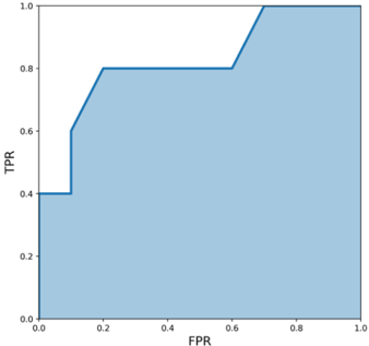
如果我们把图 3 中的表格画出来，即 TPR 在 y 轴上、FPR 在 x 轴上，我们将得到如图 4 所示的曲线。

plt.figure(figsize=(7, 7))
plt.fill_between(fpr_list, tpr_list, alpha=0.4)
plt.plot(fpr_list, tpr_list, lw=3)
plt.xlim(0, 1.0)
plt.ylim(0, 1.0)
plt.xlabel('FPR', fontsize=15)
plt.ylabel('TPR', fontsize=15)
plt.show()

FPR

Figure 4: Receiver operating characteristic (ROC) curve

这条曲线也被称为受试者工作特征（Receiver Operating Characteristic，ROC）曲线。如果我们计算这条 ROC 曲线下的面积，我们就在计算另一个指标，当你的数据集具有偏斜的二值目标时，这个指标经常被使用。

这个指标被称为 ROC 曲线下面积（Area Under ROC Curve）或曲线下面积（Area Under Curve），或者干脆叫 AUC。计算 ROC 曲线下面积的方法有很多。出于这个目的，我们将使用 scikit-learn 的出色实现。

In [X]: from sklearn import metrics
In [X]: y_true = [0, 0, 0, 0, 1, 0, 1,
...:           0, 0, 1, 0, 1, 0, 0, 1]
In [X]: y_pred = [0.1, 0.3, 0.2, 0.6, 0.8, 0.05,
...:           0.9, 0.5, 0.3, 0.66, 0.3, 0.2,
...:           0.85, 0.15, 0.99]
In [X]: metrics.roc_auc_score(y_true, y_pred)
Out[X]: 0.8300000000000001

AUC 的取值范围是 0 到 1。

AUC = 1 意味着你有一个完美的模型。大多数时候，这意味着你在验证方面犯了一些错误，应该重新审视你的数据处理和验证流程。如果你没有犯任何错误，那么恭喜你，你拥有针对你所构建模型的数据集所能拥有的最好的模型。
AUC = 0 意味着你的模型非常差（或者非常好！）。尝试反转预测的概率，例如，如果正类的概率是 \(p\)，试着用 \(1-p\) 代替它。这种 AUC 也可能意味着你的验证或数据处理有问题。
AUC = 0.5 意味着你的预测是随机的。所以，对于任何二分类问题，如果我把所有目标都预测为 0.5，我就会得到 0.5 的 AUC。

介于 0 和 0.5 之间的 AUC 值意味着你的模型比随机更差。大多数时候，这是因为你把类别搞反了。如果你尝试反转你的预测，你的 AUC 可能会大于 0.5。接近 1 的 AUC 值被认为是好的。

但是 AUC 能说明我们模型的什么呢？

假设你在构建从胸部 X 光图像检测气胸的模型时得到了 0.85 的 AUC。这意味着如果你从数据集中随机选择一张有气胸的图像（正样本）和另一张没有气胸的随机图像（负样本），那么气胸图像以 0.85 的概率排在非气胸图像前面。

选择阈值（Threshold）

在计算了概率和 AUC 之后，你会想在测试集（test set）上做预测。根据问题和用例，你可能想要概率或实际的类别。如果你想要概率，那很容易。你已经有了。如果你想要类别，你需要选择一个阈值。在二分类的情况下，你可以做如下的事情。

\[ \text{prediction} = \begin{cases} 1, & \text{if } p \geq \text{threshold} \\ 0, & \text{otherwise} \end{cases} \]

也就是说，prediction 是一个只包含二值变量的新列表。如果概率大于或等于给定的阈值，prediction 中的一项就是 1，否则值为 0。

你猜怎么着，你可以用 ROC 曲线来选择这个阈值！ROC 曲线会告诉你阈值如何影响假正例率和真正例率，从而影响假正例和真正例。你应该选择最适合你的问题和数据集的阈值。

例如，如果你不想要太多的假正例，你应该有一个较高的阈值。但是，这也会给你带来更多的假负例。观察这种权衡，选择最佳阈值。让我们看看这些阈值如何影响真正例和假正例的值。

# empty lists to store true positive
# and false positive values
tp_list = []
fp_list = []
# actual targets
y_true = [0, 0, 0, 0, 1, 0, 1, 0, 0, 1, 0, 1, 0, 0, 1]
# predicted probabilities of a sample being 1
y_pred = [0.1, 0.3, 0.2, 0.6, 0.8, 0.05, 0.9, 0.5, 0.3, 0.66, 0.3, 0.2, 0.85, 0.15, 0.99]
# some handmade thresholds
thresholds = [0, 0.1, 0.2, 0.3, 0.4, 0.5, 0.6, 0.7, 0.8, 0.85, 0.9, 0.99, 1.0]
# loop over all thresholds
for thresh in thresholds:
    # calculate predictions for a given threshold
    temp_pred = [1 if x >= thresh else 0 for x in y_pred]
    # calculate tp
    temp_tp = true_positive(y_true, temp_pred)
    # calculate fp
    temp_fp = false_positive(y_true, temp_pred)
    # append tp and fp to lists
    tp_list.append(temp_tp)
    fp_list.append(temp_fp)

利用这个，我们可以创建一个表，如图 5 所示。

Figure 5: TP and FP values for different thresholds

索引	阈值	tp	fp
0	0.00	5.0	10.0
1	0.10	5.0	9.0
2	0.20	5.0	7.0
3	0.30	4.0	6.0
4	0.40	4.0	3.0
5	0.50	4.0	3.0
6	0.60	4.0	2.0
7	0.70	3.0	1.0
8	0.80	3.0	1.0
9	0.85	2.0	1.0
10	0.90	2.0	0.0
11	0.99	1.0	0.0
12	1.00	0.0	0.0

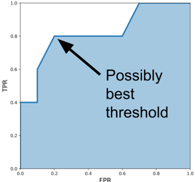
大多数时候，ROC 曲线上的左上角值应该给你一个相当好的阈值，如图 6 所示。

比较表格和 ROC 曲线，我们看到大约 0.6 的阈值相当好，我们既不会损失很多真正例，也不会有很多假正例。

FPR

Figure 6: Select the best threshold from the leftmost top point in the ROC curve

AUC 是业界广泛用于偏斜二分类任务的指标，也是每个人都应该了解的指标。一旦你理解了 AUC 背后的思想，就像上面几段解释的那样，向非技术人员解释它也容易，这些人可能在业界评估你的模型。

对数损失（Log Loss）

在学习 AUC 之后，你应该学习的另一个重要指标是对数损失（log loss）。在二分类问题的情况下，我们把对数损失定义为：

\[ \text{Log Loss} = -(y \times \log(p) + (1 - y) \times \log(1 - p)) \]

其中 target（目标）是 0 或 1，prediction（预测）是样本属于类别 1 的概率。

对于数据集中的多个样本，所有样本的对数损失只是所有单个对数损失的平均值。要记住的一点是，对数损失对错误或偏差很大的预测惩罚相当高，也就是说，对数损失会因为你非常确定但错得非常离谱而惩罚你。

import numpy as np

def log_loss(y_true, y_proba):
    """
    Function to calculate log loss
    :param y_true: list of true values
    :param y_proba: list of probabilities for 1
    :return: overall log loss
    """
    # define an epsilon value
    # this can also be an input
    # this value is used to clip probabilities
    epsilon = 1e-15
    # initialize empty list to store
    # individual losses
    loss = []
    # loop over all true and predicted probability values
    for yt, yp in zip(y_true, y_proba):
        # adjust probability
        # 0 gets converted to 1e-15
        # 1 gets converted to 1-1e-15
        # Why? Think about it!
        yp = np.clip(yp, epsilon, 1 - epsilon)
        # calculate loss for one sample
        temp_loss = - 1.0 * ( yt * np.log(yp) + (1 - yt) * np.log(1 - yp) )
        # add to loss list
        loss.append(temp_loss)
    # return mean loss over all samples
    return np.mean(loss)

让我们测试一下我们的实现：

In [X]: y_true = [0, 0, 0, 0, 1, 0, 1,
...:           0, 0, 1, 0, 1, 0, 0, 1]
In [X]: y_proba = [0.1, 0.3, 0.2, 0.6, 0.8, 0.05,
...:           0.9, 0.5, 0.3, 0.66, 0.3, 0.2,
...:           0.85, 0.15, 0.99]
In [X]: log_loss(y_true, y_proba)
Out[X]: 0.49882711861432294

我们可以与 scikit-learn 进行比较：

In [X]: from sklearn import metrics
In [X]: metrics.log_loss(y_true, y_proba)
Out[X]: 0.49882711861432294

因此，我们的实现是正确的。对数损失的实现很容易。解释可能看起来有点困难。你必须记住，对数损失的惩罚比其他指标大得多。

例如，如果你对一个样本属于类别 1 有 51% 的把握，对数损失将是：

\[ -(1 \times \log(0.51) + 0 \times \log(0.49)) = 0.6733 \]

如果你对一个样本属于类别 0 有 49% 的把握，对数损失将是：

\[ -(0 \times \log(0.51) + 1 \times \log(0.49)) = 0.7133 \]

所以，即使我们可以在 0.5 处选择一个分界点并获得完美的预测，我们仍然会有非常高的对数损失。因此，在处理对数损失时，你需要非常小心；任何不自信的预测都会有非常高的对数损失。

多分类问题的指标

到目前为止，我们讨论的大多数指标都可以转换为多分类（multi-class）版本。这个想法很简单。让我们以精确率和召回率为例。我们可以为多分类问题中的每个类别计算精确率和召回率。

有三种不同的计算方法，有时可能会让人困惑。假设我们首先对精确率感兴趣。我们知道精确率取决于真正例和假正例。

宏平均精确率（Macro averaged precision）：分别计算所有类别的精确率，然后取平均
微平均精确率（Micro averaged precision）：按类别计算真正例和假正例，然后用它们来计算总体精确率
加权精确率（Weighted precision）：与宏平均相同，但在这种情况下，它是根据每个类别中的样本数量进行的加权平均

这看起来复杂，但通过 Python 实现很容易理解。让我们看看宏平均精确率是如何实现的。

import numpy as np

def macro_precision(y_true, y_pred):
    """
    Function to calculate macro averaged precision
    :param y_true: list of true values
    :param y_pred: list of predicted values
    :return: macro precision score
    """
    # find the number of classes by taking
    # length of unique values in true list
    num_classes = len(np.unique(y_true))
    # initialize precision to 0
    precision = 0
    # loop over all classes
    for class_ in range(num_classes):
        # all classes except current are considered negative
        temp_true = [1 if p == class_ else 0 for p in y_true]
        temp_pred = [1 if p == class_ else 0 for p in y_pred]
        # calculate true positive for current class
        tp = true_positive(temp_true, temp_pred)
        # calculate false positive for current class
        fp = false_positive(temp_true, temp_pred)
        # calculate precision for current class
        temp_precision = tp / (tp + fp)
        # keep adding precision for all classes
        precision += temp_precision
    # calculate and return average precision over all classes
    precision /= num_classes
    return precision

你会注意到这并不难。同样，我们还有微平均精确率。

import numpy as np

def micro_precision(y_true, y_pred):
    """
    Function to calculate micro averaged precision
    :param y_true: list of true values
    :param y_pred: list of predicted values
    :return: micro precision score
    """
    # find the number of classes by taking
    # length of unique values in true list
    num_classes = len(np.unique(y_true))
    # initialize tp and fp to 0
    tp = 0
    fp = 0
    # loop over all classes
    for class_ in range(num_classes):
        # all classes except current are considered negative
        temp_true = [1 if p == class_ else 0 for p in y_true]
        temp_pred = [1 if p == class_ else 0 for p in y_pred]
        # calculate true positive for current class
        # and update overall tp
        tp += true_positive(temp_true, temp_pred)
        # calculate false positive for current class
        # and update overall tp
        fp += false_positive(temp_true, temp_pred)
    # calculate and return overall precision
    precision = tp / (tp + fp)
    return precision

这也不难。那什么难呢？没什么。机器学习很简单。

现在，让我们看看加权精确率的实现。

from collections import Counter
import numpy as np

def weighted_precision(y_true, y_pred):
    """
    Function to calculate weighted averaged precision
    :param y_true: list of true values
    :param y_pred: list of predicted values
    :return: weighted precision score
    """
    # find the number of classes by taking
    # length of unique values in true list
    num_classes = len(np.unique(y_true))
    # create class:sample count dictionary
    # it looks something like this:
    # {0: 20, 1:15, 2:21}
    class_counts = Counter(y_true)
    # initialize precision to 0
    precision = 0
    # loop over all classes
    for class_ in range(num_classes):
        # all classes except current are considered negative
        temp_true = [1 if p == class_ else 0 for p in y_true]
        temp_pred = [1 if p == class_ else 0 for p in y_pred]
        # calculate tp and fp for class
        tp = true_positive(temp_true, temp_pred)
        fp = false_positive(temp_true, temp_pred)
        # calculate precision of class
        temp_precision = tp / (tp + fp)
        # multiply precision with count of samples in class
        weighted_precision = class_counts[class_] * temp_precision
        # add to overall precision
        precision += weighted_precision
    # calculate overall precision by dividing by
    # total number of samples
    overall_precision = precision / len(y_true)
    return overall_precision

让我们将我们的实现与 scikit-learn 进行比较，看看我们是否实现正确。

In [X]: from sklearn import metrics
In [X]: y_true = [0, 1, 2, 0, 1, 2, 0, 2, 2]
In [X]: y_pred = [0, 2, 1, 0, 2, 1, 0, 0, 2]
In [X]: macro_precision(y_true, y_pred)
Out[X]: 0.3611111111111111
In [X]: metrics.precision_score(y_true, y_pred, average="macro")
Out[X]: 0.3611111111111111
In [X]: micro_precision(y_true, y_pred)
Out[X]: 0.4444444444444444
In [X]: metrics.precision_score(y_true, y_pred, average="micro")
Out[X]: 0.4444444444444444
In [X]: weighted_precision(y_true, y_pred)
Out[X]: 0.39814814814814814
In [X]: metrics.precision_score(y_true, y_pred, average="weighted")
Out[X]: 0.39814814814814814

看起来我们实现的一切都是正确的。请注意，这里展示的实现可能不是最高效的，但它们是最容易理解的。

同样，我们也可以为多分类实现召回率指标。精确率和召回率依赖于真正例、假正例和假负例，而 F1 依赖于精确率和召回率。

召回率的实现留给读者作为练习，这里实现了一个多分类的 F1 版本，即加权平均。

from collections import Counter
import numpy as np

def weighted_f1(y_true, y_pred):
    """
    Function to calculate weighted f1 score
    :param y_true: list of true values
    :param y_proba: list of predicted values
    :return: weighted f1 score
    """
    # find the number of classes by taking
    # length of unique values in true list
    num_classes = len(np.unique(y_true))
    # create class:sample count dictionary
    # it looks something like this:
    # {0: 20, 1:15, 2:21}
    class_counts = Counter(y_true)
    # initialize f1 to 0
    f1 = 0
    # loop over all classes
    for class_ in range(num_classes):
        # all classes except current are considered negative
        temp_true = [1 if p == class_ else 0 for p in y_true]
        temp_pred = [1 if p == class_ else 0 for p in y_pred]
        # calculate precision and recall for class
        p = precision(temp_true, temp_pred)
        r = recall(temp_true, temp_pred)
        # calculate f1 of class
        if p + r != 0:
            temp_f1 = 2 * p * r / (p + r)
        else:
            temp_f1 = 0
        # multiply f1 with count of samples in class
        weighted_f1 = class_counts[class_] * temp_f1
        # add to f1 precision
        f1 += weighted_f1
    # calculate overall F1 by dividing by
    # total number of samples
    overall_f1 = f1 / len(y_true)
    return overall_f1

请注意，上面有一些新的代码行。这就是为什么你应该仔细阅读代码。

In [X]: from sklearn import metrics
In [X]: y_true = [0, 1, 2, 0, 1, 2, 0, 2, 2]
In [X]: y_pred = [0, 2, 1, 0, 2, 1, 0, 0, 2]
In [X]: weighted_f1(y_true, y_pred)
Out[X]: 0.41269841269841273
In [X]: metrics.f1_score(y_true, y_pred, average="weighted")
Out[X]: 0.41269841269841273

因此，我们已经为多分类问题实现了精确率、召回率和 F1。你也可以类似地把 AUC 和对数损失转换为多分类格式。这种转换格式被称为一对多（one-vs-all）。我在这里不打算实现它们，因为实现与我们讨论过的非常相似。

混淆矩阵（Confusion Matrix）

在二分类或多分类中，查看混淆矩阵（confusion matrix）也很流行。别困惑；这很容易。混淆矩阵不过是一个 TP、FP、TN 和 FN 的表。使用混淆矩阵，你可以快速看到有多少样本被错误分类，有多少被正确分类。有人可能会说混淆矩阵应该在本章很早就介绍，但我选择不这样做。如果你理解 TP、FP、TN、FN、精确率、召回率和 AUC，就很容易理解和解释混淆矩阵。让我们看看二分类问题的混淆矩阵在图 7 中是什么样子的。

我们看到混淆矩阵由 TP、FP、FN 和 TN 组成。这些是我们计算精确率、召回率、F1 分数和 AUC 所需的全部值。有时，人们也喜欢把 FP 称为第一类错误（Type-I error），把 FN 称为第二类错误（Type-II error）。

预测（Predictions）

Figure 7: Confusion matrix for a binary classification task

	类别 1	类别 0
类别 1	TP	FP
类别 0	FN	TN

我们还可以把二分类混淆矩阵扩展到多分类混淆矩阵。那会是什么样子？如果我们有 N 个类别，它将是一个 NxN 大小的矩阵。对于每个类别，我们计算进入该类别和其他类别的样本总数。通过一个例子可以最好地理解这一点。

假设我们有以下真实类别（actual classes）：

\[ \text{actual} = [0, 1, 2, 0, 1, 2, 0, 2, 2] \]

而我们的预测（predictions）是：

\[ \text{predicted} = [0, 2, 1, 0, 2, 1, 0, 0, 2] \]

那么我们的混淆矩阵将如图 8 所示。

真实目标（Actual Targets）

Figure 8: Confusion matrix for a multi-class problem

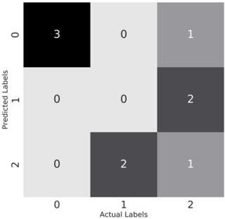
图 8 告诉了我们什么？

让我们看看类别 0。我们看到实际目标中有 3 个类别 0 的实例。然而，在预测中，有 3 个实例属于类别 0，1 个实例属于类别 1。理想情况下，对于实际标签中的类别 0，预测标签 1 和 2 不应该有任何实例。让我们看看类别 2。在实际标签中，这个计数加起来是 4，而在预测中加起来是 3。类别 2 只有 1 个实例被完美预测，2 个实例进入了类别 1。

一个完美的混淆矩阵应该只从左到右填充对角线。

混淆矩阵为计算我们之前讨论过的不同指标提供了一种简单的方法。Scikit-learn 提供了一种简单直接的方法来生成混淆矩阵。请注意，我在图 8 中展示的混淆矩阵是 scikit-learn 混淆矩阵的转置，原始版本可以用下面的代码绘制。

import matplotlib.pyplot as plt
import seaborn as sns
from sklearn import metrics
# some targets
y_true = [0, 1, 2, 0, 1, 2, 0, 2, 2]
#some predictions
y_pred = [0, 2, 1, 0, 2, 1, 0, 0, 2]
# get confusion matrix from sklearn
cm = metrics.confusion_matrix(y_true, y_pred)
# plot using matplotlib and seaborn
plt.figure(figsize=(10, 10))
cmap = sns.cubehelix_palette(50, hue=0.05, rot=0, light=0.9, dark=0, as_cmap=True)
sns.set(font_scale=2.5)
sns.heatmap(cm, annot=True, cmap=cmap, cbar=False)
plt.ylabel('Actual Labels', fontsize=20)
plt.xlabel('Predicted Labels', fontsize=20)

所以，到目前为止，我们已经处理了二分类和多分类的指标。然后是另一种类型的分类问题，叫做多标签分类（multi-label classification）。在多标签分类中，每个样本可以有一个或多个与之关联的类别。这类问题的一个简单例子是，要求你预测给定图像中的不同物体。

Figure 9: Different objects in an image 4

4 https://www.flickr.com/photos/krakluski/2950388100 License: CC BY 2.0

图 9 显示了一个知名数据集中的示例图像。请注意，这个数据集的目标是不同的，但我们不讨论这个。让我们假设目的只是预测一个物体是否存在于图像中。对于图 9，我们有一把椅子、一个花盆、一扇窗户，但我们没有其他物体，如电脑、床、电视等。所以，一张图像可以有多个与之关联的目标。这类问题就是多标签分类问题。

这类分类问题的指标有点不同。一些合适且最常见的指标是：

top-k 精确率（Precision at k，P@k）
top-k 平均精确率（Average precision at k，AP@k）
top-k 平均精确率的均值（Mean average precision at k，MAP@k）
对数损失（Log loss）

top-k 指标（P@k、AP@k、MAP@k）

让我们从 top-k 精确率或 P@k 开始。不要把这里的精确率和前面讨论的精确率混淆。如果你有一个给定样本的原始类别列表和同样的预测类别列表，精确率被定义为只考虑前 k 个预测时预测列表中的命中数除以 k。

如果这让人困惑，通过 Python 代码就会明白了。

def pk(y_true, y_pred, k):
    """
    This function calculates precision at k for a single sample
    :param y_true: list of values, actual classes
    :param y_pred: list of values, predicted classes
    :param k: the value for k
    :return: precision at a given value k
    """
    # if k is 0, return 0. we should never have this
    # as k is always >= 1
    if k == 0:
        return 0
    # we are interested only in top-k predictions
    y_pred = y_pred[:k]
    # convert predictions to set
    pred_set = set(y_pred)
    # convert actual values to set
    true_set = set(y_true)
    # find common values
    common_values = pred_set.intersection(true_set)
    # return length of common values over k
    return len(common_values) / len(y_pred[:k])

有了代码，一切都变得更容易理解。

现在，我们有 top-k 平均精确率或 AP@k。AP@k 是用 P@k 计算的。例如，如果我们要计算 AP@3，我们计算 P@1、P@2 和 P@3，然后把总和除以 3。

让我们看看它的实现。

def apk(y_true, y_pred, k):
    """
    This function calculates average precision at k for a single sample
    :param y_true: list of values, actual classes
    :param y_pred: list of values, predicted classes
    :return: average precision at a given value k
    """
    # initialize p@k list of values
    pk_values = []
    # loop over all k. from 1 to k + 1
    for i in range(1, k + 1):
        # calculate p@i and append to list
        pk_values.append(pk(y_true, y_pred, i))
    # if we have no values in the list, return 0
    if len(pk_values) == 0:
        return 0
    # else, we return the sum of list over length of list
    return sum(pk_values) / len(pk_values)

这两个函数可以用来计算两个给定列表的 top-k 平均精确率（AP@k）；让我们看看怎么做。

In [X]: y_true = [
...:     [1, 2, 3],
...:     [0, 2],
...:     [1],
...:     [2, 3],
...:     [1, 0],
...:     []
...: ]
In [X]: y_pred = [
...:     [0, 1, 2],
...:     [1],
...:     [0, 2, 3],
...:     [2, 3, 4, 0],
...:     [0, 1, 2],
...:     [0]
...: ]
In [X]: for i in range(len(y_true)):
...:     for j in range(1, 4):
...:         print(
...:             f"""
...:             y_true={y_true[i]},
...:             y_pred={y_pred[i]},
...:             AP@{j}={apk(y_true[i], y_pred[i], k=j)}
...:             """
...:         )
...: y_true=[1, 2, 3], y_pred=[0, 1, 2], AP@1=0.0
...: y_true=[1, 2, 3], y_pred=[0, 1, 2], AP@2=0.25
...: y_true=[1, 2, 3], y_pred=[0, 1, 2], AP@3=0.38888888888888884
. . .

请注意，我从输出中省略了很多值，但你明白了。所以，这就是我们如何计算每个样本的 AP@k。在机器学习中，我们对所有样本感兴趣，这就是为什么我们有 top-k 平均精确率的均值或 MAP@k。MAP@k 只是 AP@k 的平均值，可以通过下面的 Python 代码轻松计算。

def mapk(y_true, y_pred, k):
    """
    This function calculates mean avg precision at k for a single sample
    :param y_true: list of values, actual classes
    :param y_pred: list of values, predicted classes
    :return: mean avg precision at a given value k
    """
    # initialize empty list for apk values
    apk_values = []
    # loop over all samples
    for i in range(len(y_true)):
        # store apk values for every sample
        apk_values.append(
            apk(y_true[i], y_pred[i], k=k)
        )
    # return mean of apk values list
    return sum(apk_values) / len(apk_values)

现在，我们可以为同样的列表的列表计算 k=1、2、3 和 4 的 MAP@k。

In [X]: y_true = [
...:     [1, 2, 3],
...:     [0, 2],
...:     [1],
...:     [2, 3],
...:     [1, 0],
...:     []
...: ]
In [X]: y_pred = [
...:     [0, 1, 2],
...:     [1],
...:     [0, 2, 3],
...:     [2, 3, 4, 0],
...:     [0, 1, 2],
...:     [0]
...: ]
In [X]: mapk(y_true, y_pred, k=1)
Out[X]: 0.3333333333333333
In [X]: mapk(y_true, y_pred, k=2)
Out[X]: 0.375
In [X]: mapk(y_true, y_pred, k=3)
Out[X]: 0.3611111111111111
In [X]: mapk(y_true, y_pred, k=4)
Out[X]: 0.34722222222222215

P@k、AP@k 和 MAP@k 的取值范围都是从 0 到 1，1 是最好的。

请注意，有时你可能会在互联网上看到 P@k 和 AP@k 的不同实现。例如，让我们看看其中一个实现。

# taken from:
# https://github.com/benhamner/Metrics/blob/
# master/Python/ml_metrics/average_precision.py
import numpy as np

def apk(actual, predicted, k=10):
    """
    Computes the average precision at k.
    This function computes the AP at k between two lists of items.
    Parameters
    ----------
    actual : list
             A list of elements to be predicted (order doesn't matter)
    predicted : list
                A list of predicted elements (order does matter)
    k : int, optional
        The maximum number of predicted elements
    Returns
    -------
    score : double
            The average precision at k over the input lists
    """
    if len(predicted)>k:
        predicted = predicted[:k]
    score = 0.0
    num_hits = 0.0
    for i,p in enumerate(predicted):
        if p in actual and p not in predicted[:i]:
            num_hits += 1.0
            score += num_hits / (i+1.0)
    if not actual:
        return 0.0
    return score / min(len(actual), k)

这个实现是 AP@k 的另一个版本，其中顺序很重要，我们对预测进行加权。这个实现的结果与我展示的略有不同。

现在，我们来看看多标签分类的对数损失。这很容易。你可以把目标转换成二值格式，然后对每一列使用对数损失。最后，你可以取每一列对数损失的平均值。这也被称为按列平均对数损失（mean column-wise log loss）。当然，还有其他方法可以实现这一点，你应该在遇到它们时进行探索。

我们现在已经到了一个阶段，可以说我们知道了所有二分类、多分类和多标签分类指标，现在我们可以转向回归指标。

回归问题的指标

回归中最常见的指标是误差（error）。误差很简单，很容易理解。

\[ \text{Error} = \text{True Value} - \text{Predicted Value} \]

绝对误差（absolute error）就是上面这个的绝对值。

\[ \text{Absolute Error} = |\text{True Value} - \text{Predicted Value}| \]

然后是平均绝对误差（Mean Absolute Error，MAE）。它只是所有绝对误差的平均值。

import numpy as np

def mean_absolute_error(y_true, y_pred):
    """
    This function calculates mae
    :param y_true: list of real numbers, true values
    :param y_pred: list of real numbers, predicted values
    :return: mean absolute error
    """
    # initialize error at 0
    error = 0
    # loop over all samples in the true and predicted list
    for yt, yp in zip(y_true, y_pred):
        # calculate absolute error
        # and add to error
        error += np.abs(yt - yp)
    # return mean error
    return error / len(y_true)

同样，我们有平方误差和均方误差（Mean Squared Error，MSE）。

\[ \text{Squared Error} = (\text{True Value} - \text{Predicted Value})^2 \]

均方误差（MSE）可以实现如下。

def mean_squared_error(y_true, y_pred):
    """
    This function calculates mse
    :param y_true: list of real numbers, true values
    :param y_pred: list of real numbers, predicted values
    :return: mean squared error
    """
    # initialize error at 0
    error = 0
    # loop over all samples in the true and predicted list
    for yt, yp in zip(y_true, y_pred):
        # calculate squared error
        # and add to error
        error += (yt - yp) ** 2
    # return mean error
    return error / len(y_true)

MSE 和 RMSE（均方根误差，Root Mean Squared Error）是评估回归模型时最流行的指标。

\[ \text{RMSE} = \sqrt{\frac{1}{N} \sum_{i=1}^{N} (y_i - \hat{y}_i)^2} \]

同一类中的另一种误差是平方对数误差（squared logarithmic error）。有些人把它叫做 SLE，当我们对所有样本取这个误差的平均值时，它被称为 MSLE（均方对数误差，Mean Squared Logarithmic Error），实现如下。

import numpy as np

def mean_squared_log_error(y_true, y_pred):
    """
    This function calculates msle
    :param y_true: list of real numbers, true values
    :param y_pred: list of real numbers, predicted values
    :return: mean squared logarithmic error
    """
    # initialize error at 0
    error = 0
    # loop over all samples in true and predicted list
    for yt, yp in zip(y_true, y_pred):
        # calculate squared log error
        # and add to error
        error += (np.log(1 + yt) - np.log(1 + yp)) ** 2
    # return mean error
    return error / len(y_true)

均方根对数误差（Root Mean Squared Logarithmic Error）就是它的平方根。它也被称为 RMSLE。

然后是百分比误差（percentage error）：

\[ \text{Percentage Error} = \frac{\text{True Value} - \text{Predicted Value}}{\text{True Value}} \times 100 \]

同样可以转换为所有样本的平均百分比误差（Mean Percentage Error，MPE）。

def mean_percentage_error(y_true, y_pred):
    """
    This function calculates mpe
    :param y_true: list of real numbers, true values
    :param y_pred: list of real numbers, predicted values
    :return: mean percentage error
    """
    # initialize error at 0
    error = 0
    # loop over all samples in true and predicted list
    for yt, yp in zip(y_true, y_pred):
        # calculate percentage error
        # and add to error
        error += (yt - yp) / yt
    # return mean percentage error
    return error / len(y_true)

同样的绝对版本（也是更常见的版本）被称为平均绝对百分比误差（Mean Absolute Percentage Error，MAPE）。

import numpy as np

def mean_abs_percentage_error(y_true, y_pred):
    """
    This function calculates MAPE
    :param y_true: list of real numbers, true values
    :param y_pred: list of real numbers, predicted values
    :return: mean absolute percentage error
    """
    # initialize error at 0
    error = 0
    # loop over all samples in true and predicted list
    for yt, yp in zip(y_true, y_pred):
        # calculate percentage error
        # and add to error
        error += np.abs(yt - yp) / yt
    # return mean percentage error
    return error / len(y_true)

回归最好的地方在于，只有少数几个最流行的指标可以应用于几乎所有的回归问题。与分类指标相比，它也更容易理解。

R 平方（R-squared）

让我们谈谈另一个回归指标，称为 R 平方（R²，R-squared），也被称为决定系数（coefficient of determination）。

简单来说，R 平方表示你的模型对数据的拟合程度。接近 1.0 的 R 平方表示模型对数据拟合得很好，而接近 0 意味着模型不是那么好。当模型只是做出荒谬的预测时，R 平方也可能是负的。

R 平方的公式如图 10 所示，但一如既往，Python 实现会让事情更清楚。

\[ R^2 = 1 - \frac{\sum_{i=1}^{N} (y_i - \hat{y}_i)^2}{\sum_{i=1}^{N} (y_i - \bar{y})^2} \]

Figure 10: Formula for R-squared

import numpy as np

def r2(y_true, y_pred):
    """
    This function calculates r-squared score
    :param y_true: list of real numbers, true values
    :param y_pred: list of real numbers, predicted values
    :return: r2 score
    """
    # calculate the mean value of true values
    mean_true_value = np.mean(y_true)
    # initialize numerator with 0
    numerator = 0
    # initialize denominator with 0
    denominator = 0
    # loop over all true and predicted values
    for yt, yp in zip(y_true, y_pred):
        # update numerator
        numerator += (yt - yp) ** 2
        # update denominator
        denominator += (yt - mean_true_value) ** 2
    # calculate the ratio
    ratio = numerator / denominator
    # return 1 - ratio
    return 1 - ratio

评估指标还有很多，这个清单是无穷无尽的。我可以写一本只讲不同评估指标的书。也许我会的。目前，这些评估指标几乎适用于你想尝试的所有问题。请注意，我是以最直接的方式实现这些指标的，这意味着它们的效率不够高。你可以通过正确使用 numpy，把其中大多数实现得非常高效。例如，看看没有循环的平均绝对误差的实现。

import numpy as np

def mae_np(y_true, y_pred):
    return np.mean(np.abs(y_true - y_pred))

我本来可以用这种方式实现所有指标，但为了学习，最好看看底层实现。一旦你学会了纯 Python 的底层实现，并且不用太多 numpy，你就可以很容易地把它转换成 numpy，让它快得多。

高级指标

然后，还有一些高级指标。

其中一个被广泛使用的是二次加权 kappa（quadratic weighted kappa），也叫 QWK。它也被称为科恩 kappa（Cohen’s kappa）。QWK 衡量两个『评分』之间的『一致性』。评分可以是 0 到 N 之间的任何实数。预测也在同一个范围内。一致性可以被定义为这些评分彼此之间的接近程度。所以，它适用于有 N 个不同类别/类的分类问题。如果一致性高，分数就越接近 1.0。在一致性低的情况下，分数接近 0。Cohen’s kappa 在 scikit-learn 中有一个很好的实现，对这个指标的详细讨论超出了本书的范围。

In [X]: from sklearn import metrics
In [X]: y_true = [1, 2, 3, 1, 2, 3, 1, 2, 3]
In [X]: y_pred = [2, 1, 3, 1, 2, 3, 3, 1, 2]
In [X]: metrics.cohen_kappa_score(y_true, y_pred, weights="quadratic")
Out[X]: 0.33333333333333337
In [X]: metrics.accuracy_score(y_true, y_pred)
Out[X]: 0.4444444444444444

你可以看到，即使准确率很高，QWK 也更低。大于 0.85 的 QWK 被认为是非常好的！

一个重要的指标是马修斯相关系数（Matthew’s Correlation Coefficient，MCC）。MCC 的取值范围是 -1 到 1。1 是完美预测，-1 是不完美预测，0 是随机预测。MCC 的公式很简单。

\[ \text{MCC} = \frac{TP \times TN - FP \times FN}{\sqrt{(TP + FP)(TP + FN)(TN + FP)(TN + FN)}} \]

我们看到 MCC 考虑了 TP、FP、TN 和 FN，因此可以用于类别偏斜的问题。你可以用我们已经实现的东西在 Python 中快速实现它。

def mcc(y_true, y_pred):
    """
    This function calculates Matthew's Correlation Coefficient for binary classification.
    :param y_true: list of true values
    :param y_pred: list of predicted values
    :return: mcc score
    """
    tp = true_positive(y_true, y_pred)
    tn = true_negative(y_true, y_pred)
    fp = false_positive(y_true, y_pred)
    fn = false_negative(y_true, y_pred)
    numerator = (tp * tn) - (fp * fn)
    denominator = (
        (tp + fp) * (fn + tn) * (fp + tn) * (tp + fn)
    )
    denominator = denominator ** 0.5
    return numerator/denominator

这些指标可以帮助你起步，并且几乎适用于每一个机器学习问题。

要记住的一点是，为了评估无监督方法，例如某种聚类（clustering），最好创建或手动标注一个测试集，并把它与你建模部分中发生的一切分开。当你完成聚类后，你可以简单地使用任何监督学习指标在测试集上评估性能。

一旦我们理解了针对给定问题应该使用什么指标，我们就可以开始更深入地研究我们的模型以进行改进。