交叉验证
在上一章中,我们并没有构建任何模型。原因很简单:在创建任何机器学习(machine learning)模型之前,我们必须知道什么是交叉验证(cross-validation),以及如何根据你的数据集选择最合适的交叉验证方法。
那么,什么是交叉验证?我们为什么要关心它?
关于什么是交叉验证,我们可以找到多种定义。我的定义只有一句话:交叉验证是构建机器学习模型过程中的一个步骤,它帮助我们确保模型能够准确地拟合数据,同时也确保我们不会过拟合(overfitting)。但这又引出了另一个术语:过拟合(overfitting)。
为了解释过拟合,我认为最好先看一个数据集。有一个相当著名的红葡萄酒品质数据集 2。该数据集包含 11 个决定红葡萄酒品质的不同属性。
这些属性包括:
- 固定酸度(fixed acidity)
- 挥发性酸度(volatile acidity)
- 柠檬酸(citric acid)
- 残留糖分(residual sugar)
- 氯化物(chlorides)
- 游离二氧化硫(free sulfur dioxide)
- 总二氧化硫(total sulfur dioxide)
- 密度(density)
- pH
- 硫酸盐(sulphates)
- 酒精(alcohol)
基于这些不同的属性,我们需要预测红葡萄酒的品质,这是一个介于 0 到 10 之间的值。
2 P. Cortez, A. Cerdeira, F. Almeida, T. Matos and J. Reis; Modeling wine preferences by data mining from physicochemical properties. In Decision Support Systems, Elsevier, 47(4):547-553, 2009.
让我们看看这些数据长什么样。
import pandas as pd
df = pd.read_csv("winequality-red.csv")
这个数据集看起来是这样的:
Figure 1: A snapshot of the red wine quality dataset.
| 固定酸度 | 挥发性酸度 | 柠檬酸 | 残留糖分 | 氯化物 | 游离二氧化硫 | 总二氧化硫 | 密度 | pH | 硫酸盐 | 酒精 | 品质 |
|---|---|---|---|---|---|---|---|---|---|---|---|
| 6.8 | 0.67 | 0.00 | 1.9 | 0.080 | 22.0 | 39.0 | 0.99701 | 3.40 | 0.74 | 97 | 5 |
| 7.2 | 0.63 | 0.00 | 1.9 | 0.097 | 14.0 | 38.0 | 0.99675 | 3.37 | 0.58 | 0.6 | 6 |
| 8.0 | 0.31 | 0.45 | 2.1 | 0.216 | 5.0 | 16.0 | 0.99358 | 3.15 | 0.81 | 12.5 | 7 |
| 7.9 | 0.72 | 0.17 | 2.6 | 0.096 | 20.0 | 38.0 | 0.99780 | 3.40 | 0.53 | 9.5 | 5 |
| 7.6 | 0.52 | 0.12 | 3.0 | 0.067 | 12.0 | 53.0 | 0.99710 | 3.36 | 0.57 | 9.1 | 5 |
| …… | … | … | … | … | *** | … | … | … | |||
| 10.4 | 0.41 | 0.55 | 3.2 | 0.076 | 22.0 | 54.0 | 0.99960 | 3.15 | 0.89 | 6.6 | 6 |
| 9.2 | 0.59 | 0.24 | 3.3 | 0.101 | 20.0 | 47.0 | 0.99880 | 3.26 | 0.67 | 9.6 | 5 |
| 10.2 | 0.67 | 0.39 | 1.9 | 0.054 | 6.0 | 17.0 | 0.99760 | 3.17 | 0.47 | 10.0 | 5 |
| 8.1 | 0.78 | 0.10 | 3.3 | 0.090 | 4.0 | 13.0 | 0.99855 | 3.36 | 0.49 | 9.5 | 5 |
| 7.8 | 0.52 | 0.25 | 1.9 | 0.081 | 14.0 | 38.0 | 0.99840 | 3.43 | 0.65 | 0.6 | 6 |
由于葡萄酒品质本质上只是 0 到 10 之间的一个实数,我们可以把这个问题当作分类(classification)问题来处理,也可以当作回归(regression)问题来处理。为了简单起见,我们选择分类。不过,这个数据集只包含六种品质值。因此,我们将把所有品质值映射到 0 到 5。
# a mapping dictionary that maps the quality values from 0 to 5
quality_mapping = {
    3: 0,
    4: 1,
    5: 2,
    6: 3,
    7: 4,
    8: 5
}
# you can use the map function of pandas with
# any dictionary to convert the values in a given
# column to values in the dictionary
df.loc[:, "quality"] = df.quality.map(quality_mapping)
当我们审视这些数据并将其视为分类问题时,脑海中会浮现出许多可以应用的算法,也许我们可以使用神经网络(neural networks)。但如果从一开始就深入神经网络,未免有些小题大做。所以,让我们从一些简单且容易可视化的方法开始:决策树(decision trees)。
在开始理解什么是过拟合之前,让我们先把数据分成两部分。这个数据集有 1599 个样本。我们保留 1000 个样本用于训练,另外 599 个作为独立的集合。
通过下面这段代码可以很容易地完成切分:
# use sample with frac=1 to shuffle the dataframe
# we reset the indices since they change after
# shuffling the dataframe
df = df.sample(frac=1).reset_index(drop=True)

# top 1000 rows are selected
# for training
df_train = df.head(1000)

# bottom 599 values are selected
# for testing/validation
df_test = df.tail(599)
现在,我们将在训练集上训练一个决策树模型。对于决策树模型,我将使用 scikit-learn。
# import from scikit-learn
from sklearn import tree
from sklearn import metrics

# initialize decision tree classifier class
# with a max_depth of 3
clf = tree.DecisionTreeClassifier(max_depth=3)

# choose the columns you want to train on
# these are the features for the model
cols = [
    'fixed acidity',
    'volatile acidity',
    'citric acid',
    'residual sugar',
    'chlorides',
    'free sulfur dioxide',
    'total sulfur dioxide',
    'density',
    'pH',
    'sulphates',
    'alcohol'
]

# and mapped quality from before

# train the model on the provided features
clf.fit(df_train[cols], df_train.quality)
请注意,我使用了 max_depth 为 3 的决策树分类器(DecisionTreeClassifier)。这个模型的所有其他参数我都保留为默认值。
现在,我们测试该模型在训练集和测试集上的准确率(accuracy):
# generate predictions on the training set
train_predictions = clf.predict(df_train[cols])

# generate predictions on the test set
test_predictions = clf.predict(df_test[cols])

# calculate the accuracy of predictions on
# training data set
train_accuracy = metrics.accuracy_score(
    df_train.quality, train_predictions
)

# calculate the accuracy of predictions on
# test data set
test_accuracy = metrics.accuracy_score(
    df_test.quality, test_predictions
)
训练准确率和测试准确率分别为 58.9% 和 54.25%。现在我们把 max_depth 增加到 7,然后重复这个过程。得到的训练准确率为 76.6%,测试准确率为 57.3%。这里我们使用了准确率,主要是因为它是最简单直接的指标。它可能不是这个问题的最佳指标。如果我们针对不同的 max_depth 值计算这些准确率并绘制成图,会怎么样?
# NOTE: this code is written in a jupyter notebook
# import scikit-learn tree and metrics
from sklearn import tree
from sklearn import metrics

# import matplotlib and seaborn
# for plotting
import matplotlib
import matplotlib.pyplot as plt
import seaborn as sns

# this is our global size of label text
# on the plots
matplotlib.rc('xtick', labelsize=20)
matplotlib.rc('ytick', labelsize=20)

# This line ensures that the plot is displayed
# inside the notebook
%matplotlib inline

# initialize lists to store accuracies
# for training and test data
# we start with 50% accuracy
train_accuracies = [0.5]
test_accuracies = [0.5]

# iterate over a few depth values
for depth in range(1, 25):
    # init the model
    clf = tree.DecisionTreeClassifier(max_depth=depth)

    # columns/features for training
    # note that, this can be done outside
    # the loop
    cols = [
        'fixed acidity',
        'volatile acidity',
        'citric acid',
        'residual sugar',
        'chlorides',
        'free sulfur dioxide',
        'total sulfur dioxide',
        'density',
        'pH',
        'sulphates',
        'alcohol'
    ]

    # fit the model on given features
    clf.fit(df_train[cols], df_train.quality)

    # create training & test predictions
    train_predictions = clf.predict(df_train[cols])
    test_predictions = clf.predict(df_test[cols])

    # calculate training & test accuracies
    train_accuracy = metrics.accuracy_score(
        df_train.quality, train_predictions
    )
    test_accuracy = metrics.accuracy_score(
        df_test.quality, test_predictions
    )

    # append accuracies
    train_accuracies.append(train_accuracy)
    test_accuracies.append(test_accuracy)

# create two plots using matplotlib
# and seaborn
plt.figure(figsize=(10, 5))
sns.set_style("whitegrid")
plt.plot(train_accuracies, label="train accuracy")
plt.plot(test_accuracies, label="test accuracy")
plt.legend(loc="upper left", prop={'size': 15})
plt.xticks(range(0, 26, 5))
plt.xlabel("max_depth", size=20)
plt.ylabel("accuracy", size=20)
plt.show()
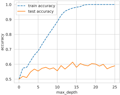
这会生成一张图,如图 2 所示。
我们看到,测试数据的最佳得分出现在 max_depth 的值为 14 的时候。随着我们不断增大这个参数的值,测试准确率保持不变或变得更差,但训练准确率却持续上升。这意味着我们简单的决策树模型随着 max_depth 的增加,对训练数据的学习越来越好,但在测试数据上的表现完全没有提升。
这就是所谓的过拟合(overfitting)。
模型在训练集上完美拟合,但在测试集上表现不佳。这意味着模型能很好地学习训练数据,却无法泛化(generalize)到未见过的样本。在上面的数据集中,人们可以构建一个 max_depth 非常高的模型,它在训练数据上会有出色的结果,但这种模型没有用处,因为它无法在真实世界样本或实时数据上给出类似的结果。
Figure 2: Training and test accuracies for different values of max_depth.
有人可能会争辩说,这种方法不算过拟合,因为测试集的准确率或多或少保持不变。过拟合的另一种定义是:当我们不断改善训练损失(loss)时,测试损失却在上升。这在神经网络中非常常见。
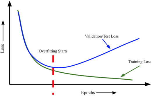
每当我们训练神经网络时,必须在训练期间同时监控训练集和测试集的损失。如果我们的网络相对于数据集来说非常大(即样本数量非常少),我们会观察到训练集和测试集的损失都会随着训练的持续而下降。然而,在某个时刻,测试损失会达到最小值,之后即使训练损失继续下降,它也会开始上升。我们必须在验证损失达到最小值的地方停止训练。
这是对过拟合最常见的解释。
奥卡姆剃刀(Occam’s razor)用简单的话说就是:不应该把可以用更简单方式解决的问题复杂化。换句话说,最简单的解决方案往往是最具泛化能力的解决方案。一般来说,每当你的模型不遵循奥卡姆剃刀原则时,它很可能就是在过拟合。
Figure 3: Most general definition of overfitting.
现在我们可以回到交叉验证了。
在解释过拟合时,我决定把数据分成两部分。我在一部分上训练模型,在另一部分上检查其表现。嗯,这也是一种交叉验证,通常称为留出集(hold-out set)。当我们有大量数据,并且模型推理(inference)是一个耗时的过程时,我们会使用这种交叉验证。
进行交叉验证的方法有很多种,而它是构建一个能够泛化到未见数据的良好机器学习模型时最关键的步骤。选择正确的交叉验证取决于你正在处理的数据集,在一个数据集上的交叉验证选择可能适用于也可能不适用于其他数据集。不过,有几种交叉验证技术是最流行、使用最广泛的。
这些方法包括:
- k 折交叉验证(k-fold cross-validation)
- 分层 k 折交叉验证(stratified k-fold cross-validation)
- 基于留出法的验证(hold-out based validation)
- 留一交叉验证(leave-one-out cross-validation)
- 组 k 折交叉验证(group k-fold cross-validation)
交叉验证就是把训练数据分成几部分。我们在其中一些部分上训练模型,在其余部分上测试。请看图 4。
Figure 4: Splitting a dataset into training and validation sets
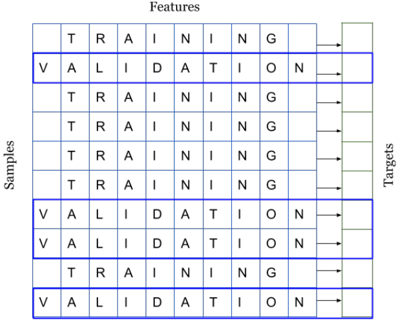
图 4 和图 5 说明:当你拿到一个用于构建机器学习模型的数据集时,你应该把它分成两个不同的集合:训练集(training set)和验证集(validation set)。也有很多人把它分成第三个集合,称为测试集(test set)。不过,我们将只使用两个集合。如你所见,我们划分样本及其对应的目标值。我们可以把数据分成 k 个互斥的不同集合。这就是所谓的 k 折交叉验证(k-fold cross-validation)。
Figure 5: K-fold cross-validation
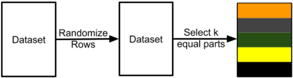
我们可以使用 scikit-learn 中的 KFold 把任何数据分成 k 个相等的部分。使用 k 折交叉验证时,每个样本都会被赋予一个 0 到 k-1 之间的值。
# import pandas and model_selection module of scikit-learn
import pandas as pd
from sklearn import model_selection

if __name__ == "__main__":
    # Training data is in a CSV file called train.csv
    df = pd.read_csv("train.csv")

    # we create a new column called kfold and fill it with -1
    df["kfold"] = -1

    # the next step is to randomize the rows of the data
    df = df.sample(frac=1).reset_index(drop=True)

    # initiate the kfold class from model_selection module
    kf = model_selection.KFold(n_splits=5)

    # fill the new kfold column
    for fold, (trn_, val_) in enumerate(kf.split(X=df)):
        df.loc[val_, 'kfold'] = fold

    # save the new csv with kfold column
    df.to_csv("train_folds.csv", index=False)
你可以把这一流程用于几乎所有类型的数据集。例如,当你有图像数据时,你可以创建一个包含图像 ID、图像位置和图像标签的 CSV,然后使用上述流程。
下一种重要的交叉验证类型是分层 k 折交叉验证(stratified k-fold cross-validation)。如果你有一个偏斜(skewed)的二分类(binary classification)数据集,其中 90% 是正样本,只有 10% 是负样本,你就不想使用随机 k 折交叉验证。对这种数据集使用简单的 k 折交叉验证,可能会导致某些折里全是负样本。在这种情况下,我们更倾向于使用分层 k 折交叉验证。分层 k 折交叉验证保持每一折中标签的比例不变。因此,在每一折中,你都会有同样的 90% 正样本和 10% 负样本。这样,无论你选择什么评估指标,它在所有折上都会给出相似的结果。
把创建 k 折交叉验证的代码修改成创建分层 k 折很容易。我们只需要把 model_selection.KFold 改成 model_selection.StratifiedKFold,并在 kf.split(...) 函数中指定我们想要分层的目标列。我们假设我们的 CSV 数据集有一个名为 ’target’ 的列,并且这是一个分类问题!
# import pandas and model_selection module of scikit-learn
import pandas as pd
from sklearn import model_selection

if __name__ == "__main__":
    # Training data is in a csv file called train.csv
    df = pd.read_csv("train.csv")

    # we create a new column called kfold and fill it with -1
    df["kfold"] = -1

    # the next step is to randomize the rows of the data
    df = df.sample(frac=1).reset_index(drop=True)

    # fetch targets
    y = df.target.values

    # initiate the kfold class from model_selection module
    kf = model_selection.StratifiedKFold(n_splits=5)

    # fill the new kfold column
    for f, (t_, v_) in enumerate(kf.split(X=df, y=y)):
        df.loc[v_, 'kfold'] = f

    # save the new csv with kfold column
    df.to_csv("train_folds.csv", index=False)
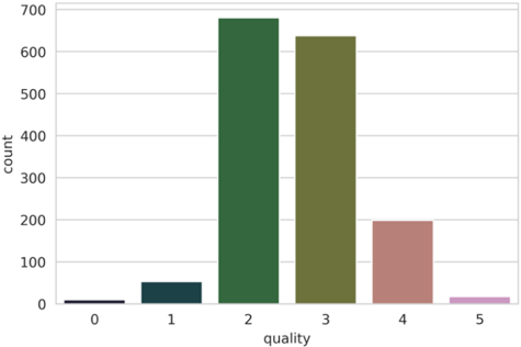
对于葡萄酒数据集,让我们看一下标签的分布。
b = sns.countplot(x='quality', data=df)
b.set_xlabel("quality", fontsize=20)
b.set_ylabel("count", fontsize=20)
请注意,我们延续上面的代码。所以,我们已经转换了目标值。看图 6,我们可以说品质(quality)是非常偏斜的。有些类别有很多样本,有些类别则没有那么多。如果我们做简单的 k 折,每一折中的目标分布不会均衡。因此,在这种情况下我们选择分层 k 折。
Figure 6: Distribution of ‘quality’ in wine dataset
规则很简单:如果是标准的分类问题,直接选择分层 k 折。
但是如果我们有大量数据该怎么办?假设我们有 100 万个样本。5 折交叉验证意味着在 80 万个样本上训练,在 20 万个样本上验证。取决于我们选择的算法,对于这种规模的数据集,训练甚至验证都可能非常昂贵。在这些情况下,我们可以选择基于留出法的验证(hold-out based validation)。
创建留出集的过程与分层 k 折相同。对于有 100 万个样本的数据集,我们可以创建 10 折而不是 5 折,并保留其中一折作为留出集。这意味着留出集中有 10 万个样本,我们将始终在这个集合上计算损失、准确率和其他指标,并在 90 万个样本上训练。
留出法也经常用于时间序列数据(time-series data)。假设我们面临的问题是预测某家商店 2020 年的销售额,而我们拥有 2015-2019 年的全部数据。在这种情况下,你可以选择 2019 年的所有数据作为留出集,并在 2015 到 2018 年的所有数据上训练你的模型。
Figure 7: Example of a time-series data
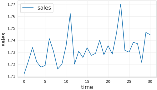
在图 7 所示的例子中,假设我们的任务是预测时间步 31 到 40 的销售额。那么我们可以把 21 到 30 作为留出集,并在第 0 步到第 20 步的数据上训练模型。你应该注意,当你在预测 31 到 40 时,应该把 21 到 30 的数据也纳入你的模型;否则性能会不尽如人意。
在很多情况下,我们不得不处理小型数据集,而创建大型验证集意味着模型会失去大量可用于学习的数据。在这些情况下,我们可以选择一种 k = N 的 k 折交叉验证,其中 N 是数据集中的样本数。这意味着在所有训练折中,我们都将在除 1 个样本之外的所有数据样本上训练。这种交叉验证的折数与数据集中的样本数相同。
应该注意的是,如果模型不够快,这种交叉验证在时间成本上可能很高,但由于这种交叉验证只适合用于小型数据集,所以关系不大。
现在我们可以转向回归问题了。回归问题的好处是,我们可以把上面提到的所有交叉验证技术都用于回归问题,除了分层 k 折。也就是说,我们不能直接使用分层 k 折,但有一些方法可以稍微改变问题,从而把分层 k 折用于回归问题。大多数情况下,简单的 k 折交叉验证适用于任何回归问题。不过,如果你发现目标分布不一致,可以使用分层 k 折。
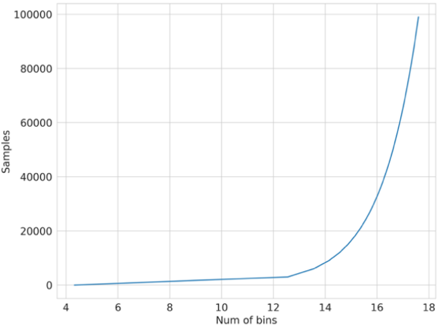
要把分层 k 折用于回归问题,我们必须先把目标值分成多个箱(bin),然后就可以像分类问题一样使用分层 k 折。关于选择合适箱数,有几种方案。如果你有大量样本(> 10k、> 100k),那么你不需要太在意箱数,直接把数据分成 10 或 20 个箱即可。如果你没有大量样本,可以使用像 Sturge 法则(Sturge’s rule)这样简单的规则来计算合适的箱数。
Sturge 法则:
\[ \text{bins} = 1 + \log_2 N \]其中 N 是数据集中的样本数。这个函数如图 8 所示。
Figure 8: Plotting samples vs the number of bins by Sturge’s Rule
让我们创建一个样本回归数据集,并尝试应用分层 k 折,如下面的 Python 代码片段所示。
# stratified-kfold for regression
import numpy as np
import pandas as pd
from sklearn import datasets
from sklearn import model_selection

def create_folds(data):
    # we create a new column called kfold and fill it with -1
    data["kfold"] = -1

    # the next step is to randomize the rows of the data
    data = data.sample(frac=1).reset_index(drop=True)

    # calculate the number of bins by Sturge's rule
    # I take the floor of the value, you can also
    # just round it
    num_bins = int(np.floor(1 + np.log2(len(data))))

    # bin targets
    data.loc[:, "bins"] = pd.cut(
        data["target"], bins=num_bins, labels=False
    )

    # initiate the kfold class from model_selection module
    kf = model_selection.StratifiedKFold(n_splits=5)

    # fill the new kfold column
    # note that, instead of targets, we use bins!
    for f, (t_, v_) in enumerate(kf.split(X=data, y=data.bins.values)):
        data.loc[v_, 'kfold'] = f

    # drop the bins column
    data = data.drop("bins", axis=1)

    # return dataframe with folds
    return data

if __name__ == "__main__":
    # we create a sample dataset with 15000 samples
    # and 100 features and 1 target
    X, y = datasets.make_regression(
        n_samples=15000, n_features=100, n_targets=1
    )

    # create a dataframe out of our numpy arrays
    df = pd.DataFrame(
        X, columns=[f"f_{i}" for i in range(X.shape[1])]
    )
    df.loc[:, "target"] = y

    # create folds
    df = create_folds(df)
在构建机器学习模型时,交叉验证是第一个也是最关键的步骤。如果你想做特征工程(feature engineering),请先切分数据。如果你打算构建模型,请先切分数据。如果你有一个良好的交叉验证方案,使验证数据能够代表训练数据和真实世界数据,你就能构建出具有高度泛化能力的良好机器学习模型。
本章介绍的交叉验证类型几乎可以应用于任何机器学习问题。不过,你必须记住,交叉验证在很大程度上也取决于数据,你可能需要根据你的问题和数据采用新的交叉验证形式。
例如,假设我们有这样一个问题:我们希望根据患者的皮肤图像构建一个检测皮肤癌的模型。我们的任务是构建一个二分类器(binary classifier),它接收一张输入图像,并预测该图像是良性(benign)还是恶性(malignant)的概率。
在这类数据集中,训练数据里同一个患者可能有多张图像。因此,要在这里构建一个良好的交叉验证系统,你必须使用分层 k 折,同时必须确保训练数据中的患者不会出现在验证数据中。幸运的是,scikit-learn 提供了一种称为 GroupKFold 的交叉验证。在这里,患者可以被视为组(groups)。但遗憾的是,在 scikit-learn 中没有办法把 GroupKFold 与 StratifiedKFold 结合起来。所以你需要自己实现。我就把它作为练习留给读者吧。